
Atomic Convolutional Networks for predicting binding affinity
Posted on * • 4 minutes • 728 words
Atomic Convolutional Networks (ACNNs)
Originally described here: https://arxiv.org/pdf/1703.10603.pdf Atomic Convolutional Networks (ACNNs) are a type of neural network architecture specifically designed for working with molecular data. ACNNs employ convolutional operations that focus on local neighborhoods of atoms within the molecule. By directly convolving over the atoms and their local connections, ACNNs can capture the spatial arrangement of atoms and the structural features of molecules effectively.
The architecture of the atomic convolutional neural network is shown below.
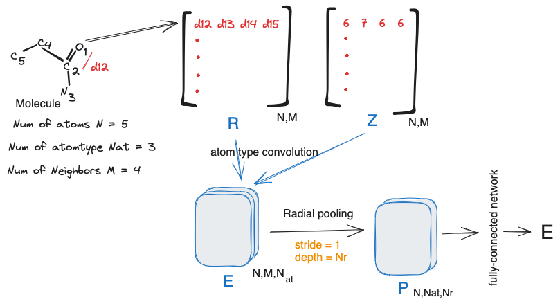
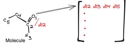
It starts with constructing distance matrix $R$ and atomic number matrix $Z$, using $M$ neighboring atoms and coordinate matrix $C$ . $R$ is a matrix where $R_{i,j} = ||C_{i} - C_{ij}||_{2}$ matrix $Z$ which lists the atomic number of neighboring atoms (atom types). $Z_{i,j} = Atom type of a_{ij}$
For atom tyoe coonvolution, $R$ is fed into a $(1 \text{x} 1)$ filter with stride 1 and depth of $N_{at}$. The atom type convolution kernel:
$ (K*R) = R_{i,j} K^{a}_{i,j} $
where
$ K^{a}{i,j} = \begin{cases} & 1 ;;; Z{i,j}=N_a\ & 0 ; \text{ otherwise } \end{cases} $
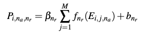
A dimensionality reduction is done with Radial Pooling layer. Importantly, radial pooling provides an output representation invariant to neighbor list atom index permutation and produces features which sum the pairwise-interactions between atom $i$ with atom type $a_i$
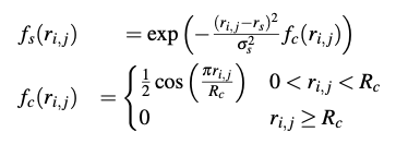
Radial pooling layers pool over slices of size $(1 \text{x} M \text{x} 1)$ with stride 1 and a depth of $N_r$, number of desired radial filters. Parameters $r_s$ and $\sigma_s$ are learnable parameters and $R_c$ is the radial interaction cutoff (=12 $\AA$)
The output P of the radial pooling layer are flattened and the tensor row-wise is fed into a fully-connected network. The same fully connected weights and biases are used for each atom in a given molecule. The output of the atomistic fully-connected network is energy $E_i$ of atom $i$. The total energy of the molecule, $E = \Sigma_i E_i$.
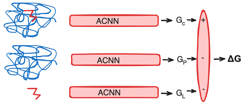
Predicting protein-ligand binding affinity
Using thermodynamic cycle:
$ \Delta G_{complex} = G_{complex} - G_{protein} - G_{ligand} $
The compnent free energies are obtained using ACNN:
Using ACNN with Deepchem
import deepchem as dc
from deepchem.molnet import load_pdbbind
from deepchem.models import AtomicConvModel
from deepchem.feat import AtomicConvFeaturizer
import os
import numpy as np
import tensorflow as tf
import matplotlib.pyplot as plt
from rdkit import Chem
!conda install -c conda-forge pycosat mdtraj pdbfixer openmm -y -q
Load Dataset and Featruize
Initialize an AtomicConvFeaturizer and load the PDBbind dataset directly using MolNet.
f1_num_atoms = 100  # maximum number of atoms to consider in the ligand
f2_num_atoms = 1000  # maximum number of atoms to consider in the protein
max_num_neighbors = 12  # maximum number of spatial neighbors for an atom

acf = AtomicConvFeaturizer(frag1_num_atoms=f1_num_atoms,
                      frag2_num_atoms=f2_num_atoms,
                      complex_num_atoms=f1_num_atoms+f2_num_atoms,
                      max_num_neighbors=max_num_neighbors,
                      neighbor_cutoff=4)
The PDBBind dataset includes experimental binding affinity data and structures for 4852 protein-ligand complexes from the “refined set” and 12800 complexes from the “general set” in PDBBind v2019 and 193 complexes from the “core set” in PDBBind v2013.
Specify to use only the binding pocket
tasks, datasets, transformers = load_pdbbind(featurizer=acf,
                                             save_dir='.',
                                             data_dir='.',
                                             pocket=True,
                                             reload=False,
                                             set_name='core')
class MyTransformer(dc.trans.Transformer):
  def transform_array(x, y, w, ids):
    kept_rows = x != None
    return x[kept_rows], y[kept_rows], w[kept_rows], ids[kept_rows],

datasets = [d.transform(MyTransformer) for d in datasets]
datasets
(<DiskDataset X.shape: (154, 9), y.shape: (154,), w.shape: (154,), ids: ['3uri' '2yki' '1ps3' ... '2d3u' '1h23' '2p4y'], task_names: [0]>,
 <DiskDataset X.shape: (19, 9), y.shape: (19,), w.shape: (19,), ids: ['3dd0' '1r5y' '3gbb' ... '2y5h' '3udh' '1w4o'], task_names: [0]>,
 <DiskDataset X.shape: (20, 9), y.shape: (20,), w.shape: (20,), ids: ['2xb8' '2r23' '2vl4' ... '2vo5' '3e93' '1loq'], task_names: [0]>)
train, val, test = datasets
Define Model and Train
the input parameters the same as those used in AtomicConvFeaturizer. layer_sizes controls the number of layers and the size of each dense layer in the network. The hyperparameters are the same as those used in the original paper .
acm = AtomicConvModel(n_tasks=1,
                      frag1_num_atoms=f1_num_atoms,
                      frag2_num_atoms=f2_num_atoms,
                      complex_num_atoms=f1_num_atoms+f2_num_atoms,
                      max_num_neighbors=max_num_neighbors,
                      batch_size=12,
                      layer_sizes=[32, 32, 16],
                      learning_rate=0.003,
                      )
losses, val_losses = [], []
%%time
max_epochs = 50

metric = dc.metrics.Metric(dc.metrics.score_function.rms_score)
step_cutoff = len(train)//12
def val_cb(model, step):
  if step%step_cutoff!=0:
      return
  val_losses.append(model.evaluate(val, metrics=[metric])['rms_score']**2)  # L2 Loss
  losses.append(model.evaluate(train, metrics=[metric])['rms_score']**2)  # L2 Loss

acm.fit(train, nb_epoch=max_epochs, max_checkpoints_to_keep=1,
                callbacks=[val_cb])
CPU times: user 46min 4s, sys: 16min 44s, total: 1h 2min 49s
Wall time: 10min 39s

0.36475067138671874
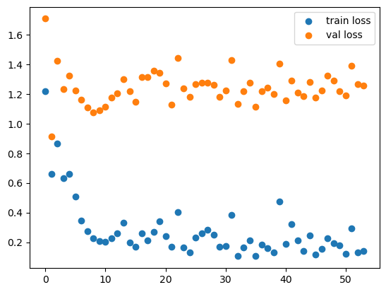
f, ax = plt.subplots()
ax.scatter(range(len(losses)), losses, label='train loss')
ax.scatter(range(len(val_losses)), val_losses, label='val loss')
plt.legend(loc='upper right');
score = dc.metrics.Metric(dc.metrics.score_function.pearson_r2_score)
for tvt, ds in zip(['train', 'val', 'test'], datasets):
  print(tvt, acm.evaluate(ds, metrics=[score]))
train {'pearson_r2_score': 0.9324012360341138}
val {'pearson_r2_score': 0.10269904927393968}
test {'pearson_r2_score': 0.14134891797477306}