

Equivariance and Invariance in GNNs
Posted on * • 11 minutes • 2307 words
Equivariance and invariance are fundamental concepts in the context of symmetries and transformations in Euclidean space.
1. Equivariance:
Equivariance refers to a property where an object’s behavior or representation changes predictably under transformations. More formally, let’s say we have two spaces $\mathbf X$ and $\mathbf Y$ and a function
$f: \mathbf X \rightarrow \mathbf Y$. If
$T_X$ and $T_Y$ are transformations on spaces
$\mathbf X$ and $\mathbf Y$ respectively, then
$f$ is equivariant with respect to $T_X$ and $T_Y$
if:
$ f \left ( T_{X} (x) \right ) = T_{Y}\left ( f(x) \right) $
This means that applying a transformation to the input and then applying the function $f$ yields the same result as applying the function $f$ and then transforming the output.
2. Invariance: Invariance refers to a property where an object’s behavior or representation remains unchanged under transformations. In other words, if we have a function $g: \mathbf X \rightarrow \mathbf Y$ and a transformation $T_X$ on space $\mathbf X$, then $g$ is invariant with respect to $T_X$ if:
$ g \left ( T_{X} (x) \right ) = g(x) $
This means that applying a transformation to the input does not change the output of the function. In the context of machine learning and neural networks, equivariance and invariance are important properties to consider when designing models that need to handle data with specific symmetries or transformations. For example, in computer vision tasks, equivariance to translation means that the network’s representation of an object should change predictably when the object is shifted in the image, while invariance to rotation means that the network’s output should remain unchanged when the object is rotated in the image.
E(3) Group: The E(3) group represents the symmetry of three-dimensional Euclidean space. It includes all possible rotations and translations in three dimensions. This group is fundamental in describing the symmetries present in 3D objects and environments.
By incorporating E(3)-invariance into the design of graph neural networks, these models can learn representations that are robust to transformations in 3D space. This can be particularly useful in applications such as 3D object recognition, molecular modeling, and computational chemistry, where understanding and exploiting 3D symmetries are crucial for accurate predictions and classifications.
import numpy as np
import matplotlib as mpl
import matplotlib.pyplot as plt
import math
import operator
from itertools import chain, product
from functools import partial
Plot a point cloud
def to_color(rgb):
  r, g, b = rgb
  return 0.1 * r + 0.8 * g + 0.1

def plot_point_cloud_3d(fig, ax_pos, color, pos, cmap='viridis', point_size=180.0, label_axes=False, annotate_points=True,
    remove_axes_ticks= True, cbar_label=""):
  cmap = mpl.cm.get_cmap(cmap)
  ax = fig.add_subplot(ax_pos, projection="3d")
  x, y, z = pos
  if remove_axes_ticks:
      ax.set_xticklabels([])
      ax.set_yticklabels([])
      ax.set_zticklabels([])
  if label_axes:
      ax.set_xlabel("$x$ coordinate")
      ax.set_ylabel("$y$ coordinate")
      ax.set_zlabel("$z$ coordinate")
  sc = ax.scatter(x, y, z, c=color, cmap=cmap, s=point_size)
  plt.colorbar(sc, location="bottom", shrink=0.6, anchor=(0.5, 2), label=cbar_label)
  if annotate_points:
      _colors = sc.cmap(color)
      rgb = _colors[:, :3].transpose()
      brightness = to_color(rgb)
      for i, (xi, yi, zi, li) in enumerate(zip(x, y, z, brightness)):
          ax.text(xi, yi, zi, str(i), None, color=[1 - li] * 3, ha="center", va="center")
  return ax
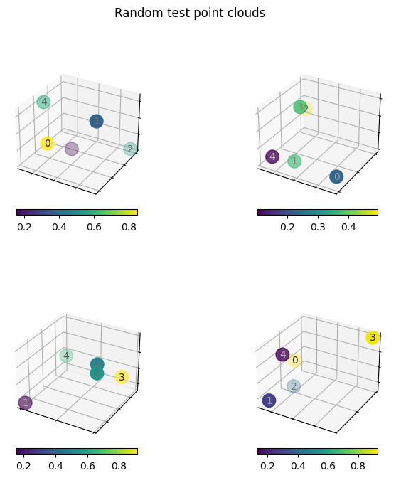
fig = plt.figure(figsize=(8, 8))

for ax_pos in [221, 222, 223, 224]:
    pos = np.random.rand(3, 5)
    color = np.random.rand(5)
    plot_point_cloud_3d(fig, ax_pos, color, pos)

fig.suptitle("Random test point clouds")
fig.tight_layout()
<ipython-input-28-447996456ece>:7: MatplotlibDeprecationWarning: The get_cmap function was deprecated in Matplotlib 3.7 and will be removed two minor releases later. Use ``matplotlib.colormaps[name]`` or ``matplotlib.colormaps.get_cmap(obj)`` instead.
  cmap = mpl.cm.get_cmap(cmap)
<ipython-input-29-95f31c0807df>:9: UserWarning: Tight layout not applied. The left and right margins cannot be made large enough to accommodate all axes decorations.
  fig.tight_layout()
import torch
import torch.nn as nn
from torch import Tensor, LongTensor
from torch_scatter import scatter
!pip install torch-scatter -f https://data.pyg.org/whl/torch-2.1.0+cu121.html
!pip install torch-geometric
import torch_geometric
from torch_geometric.transforms import BaseTransform, Compose
from torch_geometric.datasets import QM9
from torch_geometric.data import Data
from torch_geometric.loader import DataLoader
from torch_geometric.data import Dataset
from torch_geometric.nn.aggr import SumAggregation
import torch_geometric.nn as geom_nn
Functions to plot torch geometric data colored by node embeddings
from typing import Any, Optional, Callable, Tuple, Dict, Sequence, NamedTuple
def plot_model_input(data: Data, fig: mpl.figure.Figure, ax_pos: int) -> mpl.axis.Axis:
    """
    Plots 3D point cloud from torch geometric `Data` object using atomic numbers as colors.
    """
    color, pos = data.z, data.pos
    color = color.flatten().detach().numpy()
    pos = pos.T.detach().numpy()
    return plot_point_cloud_3d(fig, ax_pos, color, pos, cbar_label="Atomic number")


def plot_model_embedding(
    data: Data, model: Callable[[Data], Tensor], fig: mpl.figure.Figure, ax_pos: int
) -> mpl.axis.Axis:
    """
    Same as plot_model_input but instead of node features as color,
    from node embeddings obtained by GNN
    """
    x = model(data)
    pos = data.pos
    color = x.flatten().detach().numpy()
    pos = pos.T.detach().numpy()
    return plot_point_cloud_3d(fig, ax_pos, color, pos, cbar_label="Atom embedding (1D)")
QM9 data
from google.colab import drive
drive.mount('/content/drive')
Mounted at /content/drive
from pathlib import Path
HERE = Path(_dh[-1])
DATA = HERE / "data"
def num_heavy_atoms(qm9_data: Data) -> int:
    """Count the number of heavy atoms in a torch geometric  Data object.
    """
    # every atom with atomic number other than 1 is heavy
    return (qm9_data.z != 1).sum()


def complete_edge_index(n: int) -> LongTensor:
    """
    Constructs a complete edge index.
    """
    # filter removes self loops
    edges = list(filter(lambda e: e[0] != e[1], product(range(n), range(n))))
    return torch.tensor(edges, dtype=torch.long).T


def add_complete_graph_edge_index(data: Data) -> Data:
    """
    On top of any edge information already there,
    add a second edge index that represents
    the complete graph corresponding to a  given
    torch geometric data object
    """
    data.complete_edge_index = complete_edge_index(data.num_nodes)
    return data


#
dataset = QM9(
    DATA,
    # Filter out molecules with more than 8 heavy atoms
    pre_filter=lambda data: num_heavy_atoms(data) < 9,
    # implement point cloud adjacency as a complete graph
    pre_transform=add_complete_graph_edge_index,
)

print(f"Num. examples in QM9 restricted to molecules with at most 8 heavy atoms: {len(dataset)}")
Downloading https://data.pyg.org/datasets/qm9_v3.zip
Extracting /content/data/raw/qm9_v3.zip
Processing...
Using a pre-processed version of the dataset. Please install 'rdkit' to alternatively process the raw data.


Num. examples in QM9 restricted to molecules with at most 8 heavy atoms: 21800


Done!
Look at first molecule
data = dataset[0]
# This displays all named data attributes, and their shapes (in the case of tensors), or values (in the case of other data).
data
Data(x=[5, 11], edge_index=[2, 8], edge_attr=[8, 4], y=[1, 19], pos=[5, 3], idx=[1], name='gdb_1', z=[5], complete_edge_index=[2, 20])
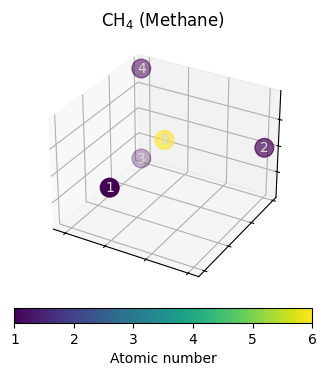
# this should be the molecule CH4
# atomic numbers stored in the attributed named z
data.z
tensor([6, 1, 1, 1, 1])
data.pos.round(decimals=2)
tensor([[-0.0100,  1.0900,  0.0100],
        [ 0.0000, -0.0100,  0.0000],
        [ 1.0100,  1.4600,  0.0000],
        [-0.5400,  1.4500, -0.8800],
        [-0.5200,  1.4400,  0.9100]])
fig = plt.figure()
ax = plot_model_input(data, fig, 111)
_ = ax.set_title("CH$_4$ (Methane)")
<ipython-input-28-447996456ece>:7: MatplotlibDeprecationWarning: The get_cmap function was deprecated in Matplotlib 3.7 and will be removed two minor releases later. Use ``matplotlib.colormaps[name]`` or ``matplotlib.colormaps.get_cmap(obj)`` instead.
  cmap = mpl.cm.get_cmap(cmap)
data module
It takes care of train/val/test splits and of indexing the correct target.
class QM9DataModule:
    def __init__(
        self,
        train_ratio: float = 0.8,
        val_ratio: float = 0.1,
        test_ratio: float = 0.1,
        target_idx: int = 5,
        seed: float = 420,
    ) -> None:
        """Encapsulates everything related to the dataset

        Parameters
        ----------
        train_ratio : float, optional
            fraction of data used for training, by default 0.8
        val_ratio : float, optional
            fraction of data used for validation, by default 0.1
        test_ratio : float, optional
            fraction of data used for testing, by default 0.1
        target_idx : int, optional
            index of the target (see torch geometric docs), by default 5 (electronic spatial extent)
            (https://pytorch-geometric.readthedocs.io/en/latest/modules/datasets.html?highlight=qm9#torch_geometric.datasets.QM9)
        seed : float, optional
            random seed for data split, by default 420
        """
        assert sum([train_ratio, val_ratio, test_ratio]) == 1
        self.target_idx = target_idx
        self.num_examples = len(self.dataset())
        rng = np.random.default_rng(seed)
        self.shuffled_index = rng.permutation(self.num_examples)
        self.train_split = self.shuffled_index[: int(self.num_examples * train_ratio)]
        self.val_split = self.shuffled_index[
            int(self.num_examples * train_ratio) : int(
                self.num_examples * (train_ratio + val_ratio)
            )
        ]
        self.test_split = self.shuffled_index[
            int(self.num_examples * (train_ratio + val_ratio)) : self.num_examples
        ]

    def dataset(self, transform=None) -> QM9:
        dataset = QM9(
            DATA,
            pre_filter=lambda data: num_heavy_atoms(data) < 9,
            pre_transform=add_complete_graph_edge_index,
        )
        dataset.data.y = dataset.data.y[:, self.target_idx].view(-1, 1)
        return dataset

    def loader(self, split, **loader_kwargs) -> DataLoader:
        dataset = self.dataset()[split]
        return DataLoader(dataset, **loader_kwargs)

    def train_loader(self, **loader_kwargs) -> DataLoader:
        return self.loader(self.train_split, shuffle=True, **loader_kwargs)

    def val_loader(self, **loader_kwargs) -> DataLoader:
        return self.loader(self.val_split, shuffle=False, **loader_kwargs)

    def test_loader(self, **loader_kwargs) -> DataLoader:
        return self.loader(self.test_split, shuffle=False, **loader_kwargs)
Non Euclidean GNN
class NaiveEuclideanGNN(nn.Module):
    def __init__(
        self,
        hidden_channels: int,
        num_layers: int,
        num_spatial_dims: int,
        final_embedding_size: Optional[int] = None,
        act: nn.Module = nn.ReLU(),
    ) -> None:
        super().__init__()
        # NOTE nn.Embedding acts like a lookup table.
        # Here we use it to store each atomic number in [0,100]
        # a learnable, fixed-size vector representation
        self.f_initial_embed = nn.Embedding(100, hidden_channels)
        self.f_pos_embed = nn.Linear(num_spatial_dims, hidden_channels)
        self.f_combine = nn.Sequential(nn.Linear(2 * hidden_channels, hidden_channels), act)

        if final_embedding_size is None:
            final_embedding_size = hidden_channels

        # Graph isomorphism network as main GNN
        # (see Talktorial 034)
        # takes care of message passing and
        # Learning node-level embeddings
        self.gnn = geom_nn.models.GIN(
            in_channels=hidden_channels,
            hidden_channels=hidden_channels,
            out_channels=final_embedding_size,
            num_layers=num_layers,
            act=act,
        )

        # modules required for aggregating node embeddings
        # into graph embeddings and making graph-level predictions
        self.aggregation = geom_nn.aggr.SumAggregation()
        self.f_predict = nn.Sequential(
            nn.Linear(final_embedding_size, final_embedding_size),
            act,
            nn.Linear(final_embedding_size, 1),
        )

    def encode(self, data: Data) -> Tensor:
        # initial atomic number embedding and embedding od positional information
        atom_embedding = self.f_initial_embed(data.z)
        pos_embedding = self.f_pos_embed(data.pos)

        # treat both as plain node-level features and combine into initial node-level
        # embedddings
        initial_node_embed = self.f_combine(torch.cat((atom_embedding, pos_embedding), dim=-1))

        # message passing
        # NOTE in contrast to the EGNN implemented later, this model does use bond information
        # i.e., data.egde_index stems from the bond adjacency matrix
        node_embed = self.gnn(initial_node_embed, data.edge_index)
        return node_embed

    def forward(self, data: Data) -> Tensor:
        node_embed = self.encode(data)
        aggr = self.aggregation(node_embed, data.batch)
        return self.f_predict(aggr)
Equivariant GNN
class EquivariantMPLayer(nn.Module):
    def __init__(
        self,
        in_channels: int,
        hidden_channels: int,
        act: nn.Module,
    ) -> None:
        super().__init__()
        self.act = act
        self.residual_proj = nn.Linear(in_channels, hidden_channels, bias=False)

        # Messages will consist of two (source and target) node embeddings and a scalar distance
        message_input_size = 2 * in_channels + 1

        # equation (3) "phi_l" NN
        self.message_mlp = nn.Sequential(
            nn.Linear(message_input_size, hidden_channels),
            act,
        )
        # equation (4) "psi_l" NN
        self.node_update_mlp = nn.Sequential(
            nn.Linear(in_channels + hidden_channels, hidden_channels),
            act,
        )

    def node_message_function(
        self,
        source_node_embed: Tensor,  # h_i
        target_node_embed: Tensor,  # h_j
        node_dist: Tensor,  # d_ij
    ) -> Tensor:
        # implements equation (3)
        message_repr = torch.cat((source_node_embed, target_node_embed, node_dist), dim=-1)
        return self.message_mlp(message_repr)

    def compute_distances(self, node_pos: Tensor, edge_index: LongTensor) -> Tensor:
        row, col = edge_index
        xi, xj = node_pos[row], node_pos[col]
        # relative squared distance
        # implements equation (2) ||X_i - X_j||^2
        rsdist = (xi - xj).pow(2).sum(1, keepdim=True)
        return rsdist

    def forward(
        self,
        node_embed: Tensor,
        node_pos: Tensor,
        edge_index: Tensor,
    ) -> Tensor:
        row, col = edge_index
        dist = self.compute_distances(node_pos, edge_index)

        # compute messages "m_ij" from  equation (3)
        node_messages = self.node_message_function(node_embed[row], node_embed[col], dist)

        # message sum aggregation in equation (4)
        aggr_node_messages = scatter(node_messages, col, dim=0, reduce="sum")

        # compute new node embeddings "h_i^{l+1}"
        # (implements rest of equation (4))
        new_node_embed = self.residual_proj(node_embed) + self.node_update_mlp(
            torch.cat((node_embed, aggr_node_messages), dim=-1)
        )

        return new_node_embed


class EquivariantGNN(nn.Module):
    def __init__(
        self,
        hidden_channels: int,
        final_embedding_size: Optional[int] = None,
        target_size: int = 1,
        num_mp_layers: int = 2,
    ) -> None:
        super().__init__()
        if final_embedding_size is None:
            final_embedding_size = hidden_channels

        # non-linear activation func.
        # usually configurable, here we just use Relu for simplicity
        self.act = nn.ReLU()

        # equation (1) "psi_0"
        self.f_initial_embed = nn.Embedding(100, hidden_channels)

        # create stack of message passing layers
        self.message_passing_layers = nn.ModuleList()
        channels = [hidden_channels] * (num_mp_layers) + [final_embedding_size]
        for d_in, d_out in zip(channels[:-1], channels[1:]):
            layer = EquivariantMPLayer(d_in, d_out, self.act)
            self.message_passing_layers.append(layer)

        # modules required for readout of a graph-level
        # representation and graph-level property prediction
        self.aggregation = SumAggregation()
        self.f_predict = nn.Sequential(
            nn.Linear(final_embedding_size, final_embedding_size),
            self.act,
            nn.Linear(final_embedding_size, target_size),
        )

    def encode(self, data: Data) -> Tensor:
        # theory, equation (1)
        node_embed = self.f_initial_embed(data.z)
        # message passing
        # theory, equation (3-4)
        for mp_layer in self.message_passing_layers:
            # NOTE here we use the complete edge index defined by the transform earlier on
            # to implement the sum over $j \neq i$ in equation (4)
            node_embed = mp_layer(node_embed, data.pos, data.complete_edge_index)
        return node_embed

    def _predict(self, node_embed, batch_index) -> Tensor:
        aggr = self.aggregation(node_embed, batch_index)
        return self.f_predict(aggr)

    def forward(self, data: Data) -> Tensor:
        node_embed = self.encode(data)
        pred = self._predict(node_embed, data.batch)
        return pred
Build a rotation matrix
Function to rotate a sample molecule. Take a sample data, clone it and rotate it.
# use rotations along z-axis as demo e(3) transformation
def rotation_matrix_z(theta: float) -> Tensor:
    """Generates a rotation matrix and returns
    a corresponing tensor. The rotation is about the $z$-axis.
    """
    return torch.tensor(
        [
            [math.cos(theta), -math.sin(theta), 0],
            [math.sin(theta), math.cos(theta), 0],
            [0, 0, 1],
        ]
    )

# Some data points from qm9
sample_data = dataset[800].clone()

# apply an E(3) transformation
rotated_sample_data = sample_data.clone()
rotated_sample_data.pos = rotated_sample_data.pos @ rotation_matrix_z(45)
Run Non Eucledian GNN
Then pass sample data and rotated data through a plain GNN
# initialize a model with 2 hidden layers, 32 hidden channels,
# that outputs 1-dimensional node embeddings
model = NaiveEuclideanGNN(
    hidden_channels=32,
    num_layers=2,
    num_spatial_dims=3,
    final_embedding_size=1,
)

# make a plot that demonstrates non-equivariance
# fig, axes = plt.subplots(2, 2, figsize=(8,8), sharex=True, sharey=True)
fig = plt.figure(figsize=(8, 8))

ax1 = plot_model_input(sample_data, fig, 221)
ax1.set_title("Sample input $(X, Z)$")

ax2 = plot_model_input(rotated_sample_data, fig, 222)
ax2.set_title("Rotated input $(X, g(Z))$")

ax3 = plot_model_embedding(sample_data, model.encode, fig, 223)
ax3.set_title("Model output for $(X, Z)$")

ax4 = plot_model_embedding(rotated_sample_data, model.encode, fig, 224)
ax4.set_title("Model output for $(X, g(Z))$")
fig.tight_layout()
<ipython-input-28-447996456ece>:7: MatplotlibDeprecationWarning: The get_cmap function was deprecated in Matplotlib 3.7 and will be removed two minor releases later. Use ``matplotlib.colormaps[name]`` or ``matplotlib.colormaps.get_cmap(obj)`` instead.
  cmap = mpl.cm.get_cmap(cmap)
<ipython-input-54-017978f0cde7>:25: UserWarning: Tight layout not applied. The left and right margins cannot be made large enough to accommodate all axes decorations.
  fig.tight_layout()
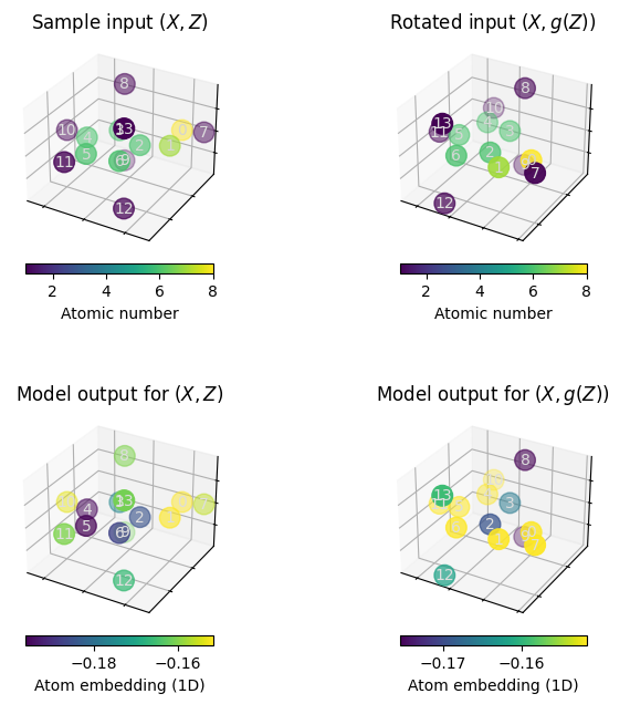
When executing the above cells a few times, we can observe that rotating the molecule may significantly alter the atom embeddings obtained from the plain GNN model.
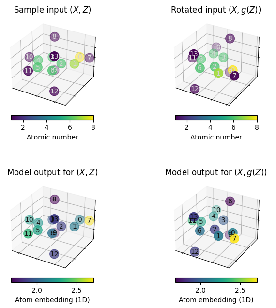
Run a Eucledian GNN
model = EquivariantGNN(hidden_channels=32, final_embedding_size=1, num_mp_layers=2)

fig = plt.figure(figsize=(8, 8))

ax1 = plot_model_input(sample_data, fig, 221)
ax1.set_title("Sample input $(X, Z)$")

ax2 = plot_model_input(rotated_sample_data, fig, 222)
ax2.set_title("Rotated input $(X, g(Z))$")

ax3 = plot_model_embedding(sample_data, model.encode, fig, 223)
ax3.set_title("Model output for $(X, Z)$")

ax4 = plot_model_embedding(rotated_sample_data, model.encode, fig, 224)
ax4.set_title("Model output for $(X, g(Z))$")
fig.tight_layout()
<ipython-input-28-447996456ece>:7: MatplotlibDeprecationWarning: The get_cmap function was deprecated in Matplotlib 3.7 and will be removed two minor releases later. Use ``matplotlib.colormaps[name]`` or ``matplotlib.colormaps.get_cmap(obj)`` instead.
  cmap = mpl.cm.get_cmap(cmap)
<ipython-input-61-d9b099a18db3>:16: UserWarning: Tight layout not applied. The left and right margins cannot be made large enough to accommodate all axes decorations.
  fig.tight_layout()
Reference:
-
E(n)-Equivariant Graph Neural Networks: International conference on machine learning (2021), 139.
-
Talktorial T036 by Volkamer lab