Attribuiton - GNN expalanation
Posted on * • 12 minutes • 2483 words
Attribution in the context of GNNs refers to understanding the importance or relevance of different nodes, edges, or subgraphs in the input graph concerning the output of the network. It aims to answer questions such as: “Why did the model make this prediction?” or “Which parts of the graph contributed the most to the final decision?” Understanding attribution is crucial for interpreting the behavior of GNNs, debugging models, and gaining insights into the underlying data.
Here’s how attribution techniques can be applied to GNNs:
- Node-level attribution: This involves understanding the importance of individual nodes in the graph. Techniques such as Gradient-based methods, Integrated Gradients, or Randomized algorithms can be used to compute the contribution of each node to the final prediction. For example, in a social network, node-level attribution could help identify influential users or communities.
- Edge-level attribution: Similarly, understanding the importance of edges in the graph can provide insights into the relationships between nodes. Techniques such as edge gradients or edge saliency maps can be employed to assess the impact of each edge on the model’s output. This could be useful in applications such as fraud detection in financial networks or identifying critical connections in transportation networks.
- Subgraph-level attribution: In some cases, attributing importance to subgraphs (i.e., groups of nodes and edges) might be more meaningful than analyzing individual nodes or edges. Techniques such as graph attention mechanisms or subgraph saliency methods can be used to identify significant substructures within the graph and their contributions to the overall prediction. For example, in molecular graphs, identifying important substructures could aid in drug discovery.
- Visualization and Interpretation: Attribution methods can also be used to visualize and interpret the decisions made by GNNs. By highlighting the most influential nodes or edges in the graph, these techniques can provide human-interpretable explanations for the model’s behavior, making it easier to understand and trust the predictions.
Overall, attribution techniques play a vital role in interpreting the behavior of GNNs and understanding how they leverage the underlying graph structure to make predictions. These methods enable users to gain insights into the model’s decision-making process and facilitate trust, transparency, and interpretability in graph-based machine learning applications.
# Install required packages.
import os
import torch
os.environ['TORCH'] = torch.__version__
print(torch.__version__)

!pip install -q torch-scatter -f https://data.pyg.org/whl/torch-${TORCH}.html
!pip install -q torch-sparse -f https://data.pyg.org/whl/torch-${TORCH}.html
!pip install -q git+https://github.com/pyg-team/pytorch_geometric.git
!pip install -q captum

# Helper function for visualization.
%matplotlib inline
import matplotlib.pyplot as plt
1.11.0+cu113
[K |████████████████████████████████| 7.9 MB 7.8 MB/s
[K |████████████████████████████████| 3.5 MB 9.8 MB/s
[?25h Building wheel for torch-geometric (setup.py) ... [?25l[?25hdone
[K |████████████████████████████████| 1.4 MB 10.2 MB/s
[?25h
Explaining GNN Model Predictions using Captum
Lets see how to apply feature attribution methods to graphs. Specifically, we try to find the most important edges for each instance prediction.
We use the Mutagenicity dataset from TUDatasets. This dataset consists of 4337 molecule graphs where the task is to predict the molecule mutagenicity.
Loading the dataset
We load the dataset and use 10% of the data as the test split.
from torch_geometric.loader import DataLoader
from torch_geometric.datasets import TUDataset

path = '.'
dataset = TUDataset(path, name='Mutagenicity').shuffle()
test_dataset = dataset[:len(dataset) // 10]
train_dataset = dataset[len(dataset) // 10:]
test_loader = DataLoader(test_dataset, batch_size=128)
train_loader = DataLoader(train_dataset, batch_size=128)
Downloading https://www.chrsmrrs.com/graphkerneldatasets/Mutagenicity.zip
Extracting ./Mutagenicity/Mutagenicity.zip
Processing...
Done!
Visualizing the data
We define some utility functions for visualizing the molecules and draw a random molecule.
import networkx as nx
import numpy as np

from torch_geometric.utils import to_networkx


def draw_molecule(g, edge_mask=None, draw_edge_labels=False):
    g = g.copy().to_undirected()
    node_labels = {}
    for u, data in g.nodes(data=True):
        node_labels[u] = data['name']
    pos = nx.planar_layout(g)
    pos = nx.spring_layout(g, pos=pos)
    if edge_mask is None:
        edge_color = 'black'
        widths = None
    else:
        edge_color = [edge_mask[(u, v)] for u, v in g.edges()]
        widths = [x * 10 for x in edge_color]
    nx.draw(g, pos=pos, labels=node_labels, width=widths,
            edge_color=edge_color, edge_cmap=plt.cm.Blues,
            node_color='azure')

    if draw_edge_labels and edge_mask is not None:
        edge_labels = {k: ('%.2f' % v) for k, v in edge_mask.items()}
        nx.draw_networkx_edge_labels(g, pos, edge_labels=edge_labels,
                                    font_color='red')
    plt.show()


def to_molecule(data):
    ATOM_MAP = ['C', 'O', 'Cl', 'H', 'N', 'F',
                'Br', 'S', 'P', 'I', 'Na', 'K', 'Li', 'Ca']
    g = to_networkx(data, node_attrs=['x'])
    for u, data in g.nodes(data=True):
        data['name'] = ATOM_MAP[data['x'].index(1.0)]
        del data['x']
    return g
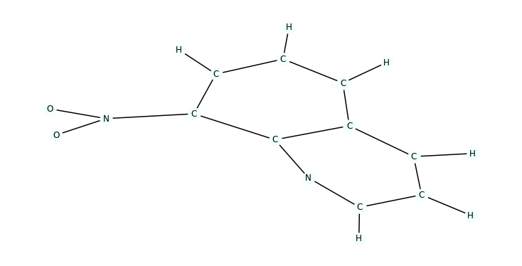
Sample visualization
We sample a single molecule from train_dataset and visualize it
import random

data = random.choice([t for t in train_dataset])
mol = to_molecule(data)
plt.figure(figsize=(10, 5))
draw_molecule(mol)
Training the model
In the next section, we train a GNN model with 5 convolution layers. We use GraphConv which supports edge_weight as a parameter. Many convolution layers in Pytorch Geometric supoort this argument.
Define the model
import torch
from torch.nn import Linear
import torch.nn.functional as F

from torch_geometric.nn import GraphConv, global_add_pool

class Net(torch.nn.Module):
    def __init__(self, dim):
        super(Net, self).__init__()

        num_features = dataset.num_features
        self.dim = dim

        self.conv1 = GraphConv(num_features, dim)
        self.conv2 = GraphConv(dim, dim)
        self.conv3 = GraphConv(dim, dim)
        self.conv4 = GraphConv(dim, dim)
        self.conv5 = GraphConv(dim, dim)

        self.lin1 = Linear(dim, dim)
        self.lin2 = Linear(dim, dataset.num_classes)

    def forward(self, x, edge_index, batch, edge_weight=None):
        x = self.conv1(x, edge_index, edge_weight).relu()
        x = self.conv2(x, edge_index, edge_weight).relu()
        x = self.conv3(x, edge_index, edge_weight).relu()
        x = self.conv4(x, edge_index, edge_weight).relu()
        x = self.conv5(x, edge_index, edge_weight).relu()
        x = global_add_pool(x, batch)
        x = self.lin1(x).relu()
        x = F.dropout(x, p=0.5, training=self.training)
        x = self.lin2(x)
        return F.log_softmax(x, dim=-1)
Define train and test functions
def train(epoch):
    model.train()

    if epoch == 51:
        for param_group in optimizer.param_groups:
            param_group['lr'] = 0.5 * param_group['lr']

    loss_all = 0
    for data in train_loader:
        data = data.to(device)
        optimizer.zero_grad()
        output = model(data.x, data.edge_index, data.batch)
        loss = F.nll_loss(output, data.y)
        loss.backward()
        loss_all += loss.item() * data.num_graphs
        optimizer.step()
    return loss_all / len(train_dataset)


def test(loader):
    model.eval()

    correct = 0
    for data in loader:
        data = data.to(device)
        output = model(data.x, data.edge_index, data.batch)
        pred = output.max(dim=1)[1]
        correct += pred.eq(data.y).sum().item()
    return correct / len(loader.dataset)
Train the model for 100 epochs
The accuracy should be around 80% in the end
device = torch.device('cuda' if torch.cuda.is_available() else 'cpu')
model = Net(dim=32).to(device)
optimizer = torch.optim.Adam(model.parameters(), lr=0.001)

for epoch in range(1, 101):
    loss = train(epoch)
    train_acc = test(train_loader)
    test_acc = test(test_loader)
    print(f'Epoch: {epoch:03d}, Loss: {loss:.4f}, '
          f'Train Acc: {train_acc:.4f}, Test Acc: {test_acc:.4f}')
Epoch: 001, Loss: 0.7441, Train Acc: 0.5904, Test Acc: 0.5473
Epoch: 002, Loss: 0.6459, Train Acc: 0.6550, Test Acc: 0.6328
Epoch: 003, Loss: 0.6112, Train Acc: 0.7018, Test Acc: 0.6975
Epoch: 004, Loss: 0.5862, Train Acc: 0.7152, Test Acc: 0.7136
Epoch: 005, Loss: 0.5750, Train Acc: 0.7318, Test Acc: 0.7206
Epoch: 006, Loss: 0.5557, Train Acc: 0.7392, Test Acc: 0.7390
Epoch: 007, Loss: 0.5473, Train Acc: 0.7464, Test Acc: 0.7367
Epoch: 008, Loss: 0.5433, Train Acc: 0.7403, Test Acc: 0.7321
Epoch: 009, Loss: 0.5469, Train Acc: 0.7551, Test Acc: 0.7483
Epoch: 010, Loss: 0.5243, Train Acc: 0.7779, Test Acc: 0.7483
Epoch: 011, Loss: 0.5178, Train Acc: 0.7772, Test Acc: 0.7529
Epoch: 012, Loss: 0.4972, Train Acc: 0.7787, Test Acc: 0.7575
Epoch: 013, Loss: 0.4926, Train Acc: 0.7797, Test Acc: 0.7529
Epoch: 014, Loss: 0.4908, Train Acc: 0.7900, Test Acc: 0.7852
Epoch: 015, Loss: 0.4843, Train Acc: 0.7971, Test Acc: 0.7552
Epoch: 016, Loss: 0.4906, Train Acc: 0.7825, Test Acc: 0.7483
Epoch: 017, Loss: 0.4744, Train Acc: 0.8048, Test Acc: 0.7737
Epoch: 018, Loss: 0.4581, Train Acc: 0.8069, Test Acc: 0.7691
Epoch: 019, Loss: 0.4522, Train Acc: 0.8110, Test Acc: 0.7737
Epoch: 020, Loss: 0.4546, Train Acc: 0.8071, Test Acc: 0.7968
Epoch: 021, Loss: 0.4520, Train Acc: 0.8110, Test Acc: 0.7598
Epoch: 022, Loss: 0.4441, Train Acc: 0.8148, Test Acc: 0.7829
Epoch: 023, Loss: 0.4572, Train Acc: 0.8015, Test Acc: 0.7783
Epoch: 024, Loss: 0.4407, Train Acc: 0.8215, Test Acc: 0.7783
Epoch: 025, Loss: 0.4382, Train Acc: 0.8153, Test Acc: 0.7806
Epoch: 026, Loss: 0.4296, Train Acc: 0.8240, Test Acc: 0.7829
Epoch: 027, Loss: 0.4234, Train Acc: 0.8158, Test Acc: 0.7829
Epoch: 028, Loss: 0.4233, Train Acc: 0.8163, Test Acc: 0.7829
Epoch: 029, Loss: 0.4221, Train Acc: 0.8112, Test Acc: 0.7829
Epoch: 030, Loss: 0.4138, Train Acc: 0.8227, Test Acc: 0.7829
Epoch: 031, Loss: 0.4158, Train Acc: 0.8199, Test Acc: 0.7737
Epoch: 032, Loss: 0.4070, Train Acc: 0.8289, Test Acc: 0.7852
Epoch: 033, Loss: 0.4043, Train Acc: 0.8202, Test Acc: 0.7852
Epoch: 034, Loss: 0.4047, Train Acc: 0.8263, Test Acc: 0.7945
Epoch: 035, Loss: 0.4024, Train Acc: 0.8181, Test Acc: 0.7875
Epoch: 036, Loss: 0.4050, Train Acc: 0.8376, Test Acc: 0.7945
Epoch: 037, Loss: 0.3865, Train Acc: 0.8363, Test Acc: 0.7945
Epoch: 038, Loss: 0.3889, Train Acc: 0.8274, Test Acc: 0.7945
Epoch: 039, Loss: 0.3964, Train Acc: 0.8176, Test Acc: 0.7991
Epoch: 040, Loss: 0.3856, Train Acc: 0.8407, Test Acc: 0.8199
Epoch: 041, Loss: 0.3877, Train Acc: 0.8391, Test Acc: 0.8037
Epoch: 042, Loss: 0.3901, Train Acc: 0.8448, Test Acc: 0.7991
Epoch: 043, Loss: 0.3802, Train Acc: 0.8448, Test Acc: 0.7991
Epoch: 044, Loss: 0.3781, Train Acc: 0.8363, Test Acc: 0.8037
Epoch: 045, Loss: 0.3817, Train Acc: 0.8543, Test Acc: 0.8176
Epoch: 046, Loss: 0.3673, Train Acc: 0.8491, Test Acc: 0.8152
Epoch: 047, Loss: 0.3666, Train Acc: 0.8409, Test Acc: 0.8152
Epoch: 048, Loss: 0.3729, Train Acc: 0.8430, Test Acc: 0.8060
Epoch: 049, Loss: 0.3651, Train Acc: 0.8484, Test Acc: 0.8176
Epoch: 050, Loss: 0.3740, Train Acc: 0.8522, Test Acc: 0.8129
Epoch: 051, Loss: 0.3615, Train Acc: 0.8578, Test Acc: 0.8014
Epoch: 052, Loss: 0.3554, Train Acc: 0.8632, Test Acc: 0.8060
Epoch: 053, Loss: 0.3490, Train Acc: 0.8607, Test Acc: 0.7921
Epoch: 054, Loss: 0.3427, Train Acc: 0.8642, Test Acc: 0.8083
Epoch: 055, Loss: 0.3324, Train Acc: 0.8635, Test Acc: 0.7898
Epoch: 056, Loss: 0.3350, Train Acc: 0.8681, Test Acc: 0.8106
Epoch: 057, Loss: 0.3296, Train Acc: 0.8704, Test Acc: 0.8152
Epoch: 058, Loss: 0.3381, Train Acc: 0.8642, Test Acc: 0.8245
Epoch: 059, Loss: 0.3298, Train Acc: 0.8683, Test Acc: 0.8152
Epoch: 060, Loss: 0.3284, Train Acc: 0.8712, Test Acc: 0.8152
Epoch: 061, Loss: 0.3288, Train Acc: 0.8660, Test Acc: 0.8014
Epoch: 062, Loss: 0.3295, Train Acc: 0.8701, Test Acc: 0.8014
Epoch: 063, Loss: 0.3274, Train Acc: 0.8637, Test Acc: 0.7921
Epoch: 064, Loss: 0.3284, Train Acc: 0.8681, Test Acc: 0.8014
Epoch: 065, Loss: 0.3278, Train Acc: 0.8632, Test Acc: 0.7945
Epoch: 066, Loss: 0.3222, Train Acc: 0.8645, Test Acc: 0.7968
Epoch: 067, Loss: 0.3249, Train Acc: 0.8730, Test Acc: 0.7991
Epoch: 068, Loss: 0.3107, Train Acc: 0.8717, Test Acc: 0.8014
Epoch: 069, Loss: 0.3219, Train Acc: 0.8760, Test Acc: 0.7968
Epoch: 070, Loss: 0.3127, Train Acc: 0.8763, Test Acc: 0.8060
Epoch: 071, Loss: 0.3111, Train Acc: 0.8799, Test Acc: 0.8060
Epoch: 072, Loss: 0.3119, Train Acc: 0.8599, Test Acc: 0.8060
Epoch: 073, Loss: 0.3134, Train Acc: 0.8696, Test Acc: 0.7921
Epoch: 074, Loss: 0.3067, Train Acc: 0.8770, Test Acc: 0.7991
Epoch: 075, Loss: 0.3108, Train Acc: 0.8768, Test Acc: 0.7968
Epoch: 076, Loss: 0.3090, Train Acc: 0.8809, Test Acc: 0.7991
Epoch: 077, Loss: 0.3002, Train Acc: 0.8791, Test Acc: 0.8014
Epoch: 078, Loss: 0.3116, Train Acc: 0.8699, Test Acc: 0.7875
Epoch: 079, Loss: 0.3068, Train Acc: 0.8753, Test Acc: 0.7921
Epoch: 080, Loss: 0.3019, Train Acc: 0.8760, Test Acc: 0.7991
Epoch: 081, Loss: 0.3026, Train Acc: 0.8691, Test Acc: 0.7829
Epoch: 082, Loss: 0.2940, Train Acc: 0.8768, Test Acc: 0.7968
Epoch: 083, Loss: 0.2946, Train Acc: 0.8783, Test Acc: 0.8152
Epoch: 084, Loss: 0.2936, Train Acc: 0.8827, Test Acc: 0.8060
Epoch: 085, Loss: 0.2945, Train Acc: 0.8747, Test Acc: 0.8014
Epoch: 086, Loss: 0.2948, Train Acc: 0.8735, Test Acc: 0.7875
Epoch: 087, Loss: 0.2940, Train Acc: 0.8801, Test Acc: 0.8060
Epoch: 088, Loss: 0.2905, Train Acc: 0.8842, Test Acc: 0.8060
Epoch: 089, Loss: 0.3051, Train Acc: 0.8614, Test Acc: 0.8222
Epoch: 090, Loss: 0.3221, Train Acc: 0.8699, Test Acc: 0.7968
Epoch: 091, Loss: 0.2995, Train Acc: 0.8809, Test Acc: 0.8037
Epoch: 092, Loss: 0.2845, Train Acc: 0.8886, Test Acc: 0.8176
Epoch: 093, Loss: 0.2907, Train Acc: 0.8899, Test Acc: 0.8152
Epoch: 094, Loss: 0.2846, Train Acc: 0.8837, Test Acc: 0.7991
Epoch: 095, Loss: 0.2774, Train Acc: 0.8878, Test Acc: 0.8060
Epoch: 096, Loss: 0.2893, Train Acc: 0.8824, Test Acc: 0.7921
Epoch: 097, Loss: 0.2769, Train Acc: 0.8870, Test Acc: 0.7991
Epoch: 098, Loss: 0.2789, Train Acc: 0.8919, Test Acc: 0.8060
Epoch: 099, Loss: 0.2794, Train Acc: 0.8901, Test Acc: 0.8037
Epoch: 100, Loss: 0.2770, Train Acc: 0.8852, Test Acc: 0.7945
Explaining the predictions
Now we look at two popular attribution methods. First, we calculate the gradient of the output with respect to the edge weights $w_{e_i}$. Edge weights are initially one for all edges. For the saliency method, we use the absolute value of the gradient as the attribution value for each edge:
$$ Attribution_{e_i} = |\frac{\partial F(x)}{\partial w_{e_i}}| $$
Where $x$ is the input and $F(x)$ is the output of the GNN model on input $x$.
For Integrated Gradients method, we interpolate between the current input and a baseline input where the weight of all edges is zero and accumulate the gradient values for each edge:
$$ Attribution_{e_i} = \int_{\alpha =0}^1 \frac{\partial F(x_{\alpha)}}{\partial w_{e_i}} d\alpha $$
Where $x_{\alpha}$ is the same as the original input graph but the weight of all edges is set to $\alpha$. Integrated Gradients complete formulation is more complicated but since our initial edge weights are equal to one and the baseline is zero, it can be simplified to the formulation above. You can read more about this method here. Of course, this can not be calculated directly and is approximated by a discrete sum.
We use the captum library for calculating the attribution values. We define the model_forward function which calculates the batch argument assuming that we are only explaining a single graph at a time.
from captum.attr import Saliency, IntegratedGradients

def model_forward(edge_mask, data):
    batch = torch.zeros(data.x.shape[0], dtype=int).to(device)
    out = model(data.x, data.edge_index, batch, edge_mask)
    return out


def explain(method, data, target=0):
    input_mask = torch.ones(data.edge_index.shape[1]).requires_grad_(True).to(device)
    if method == 'ig':
        ig = IntegratedGradients(model_forward)
        mask = ig.attribute(input_mask, target=target,
                            additional_forward_args=(data,),
                            internal_batch_size=data.edge_index.shape[1])
    elif method == 'saliency':
        saliency = Saliency(model_forward)
        mask = saliency.attribute(input_mask, target=target,
                                  additional_forward_args=(data,))
    else:
        raise Exception('Unknown explanation method')

    edge_mask = np.abs(mask.cpu().detach().numpy())
    if edge_mask.max() > 0:  # avoid division by zero
        edge_mask = edge_mask / edge_mask.max()
    return edge_mask
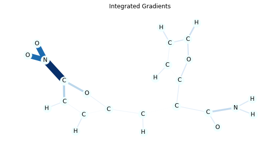
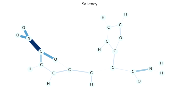
Finally we take a random sample from the test dataset and run the explanation methods. For a simpler visualization, we make the graph undirected and merge the explanations of each edge in both directions.
It is known that NO2 substructure makes the molecules mutagenic in many cases and you can verify this by the model explanations.
Mutagenic molecules have label 0 in this dataset and we only sample from those molecules but you can change the code and see the explanations for the other class as well.
In this visualization, edge colors and thickness represent the importance. You can also see the numeric value by passing draw_edge_labels to draw_molecule function.
As you can see Integrated Gradients tend to create more accurate explanations.
import random
from collections import defaultdict

def aggregate_edge_directions(edge_mask, data):
    edge_mask_dict = defaultdict(float)
    for val, u, v in list(zip(edge_mask, *data.edge_index)):
        u, v = u.item(), v.item()
        if u > v:
            u, v = v, u
        edge_mask_dict[(u, v)] += val
    return edge_mask_dict


data = random.choice([t for t in test_dataset if not t.y.item()])
mol = to_molecule(data)

for title, method in [('Integrated Gradients', 'ig'), ('Saliency', 'saliency')]:
    edge_mask = explain(method, data, target=0)
    edge_mask_dict = aggregate_edge_directions(edge_mask, data)
    plt.figure(figsize=(10, 5))
    plt.title(title)
    draw_molecule(mol, edge_mask_dict)