
Gaussian Process
Posted on * • 4 minutes • 675 words
Like a Gaussian distribution is a distribution over vectors, A GP is a Gaussian distribution over functions. Here, the aim is to learn a function. In a probabilistic linear regression problem: $y_{i}=\alpha+\beta x_{i}+\epsilon$
$Y$ is a linear function $f(X)$ parametrized by $\alpha,\beta,$ and $\sigma$
$$ \mu_{i}=\alpha+\beta x_{i} $$ $$ y_{i}\sim \mathcal{N}(\mu_{i},\sigma) $$
A Gaussian process is closely related to Bayesian linear regression. Gaussian process places a distribution directly on the space of functions $f(x)$. And like Bayesian methods a GP defines a prior over functions, which can be converted into a posterior over functions once we have seen some data.
It is a non-parametric, Bayesian approach that can be applied to supervised learning problems like regression and classification. GP has several practical advantages: it can work well on small datasets and can provide uncertainty measurements on the predictions.
Multivariate Gaussian Distribution
First, lets review the mathematical concepts.
A Gaussian random variable $X\backsim\mathcal{{N}}(\mu,\Sigma)$, where $\mu$ is the mean and $\Sigma$ is the covariance matrix has the following probability density function:
$$ P(x;\mu,\Sigma)=\frac{1}{(2\pi)^{d/2}}exp(-\frac{1}{2}(x-\mu)^{T}\Sigma^{-1}(x-\mu)) $$
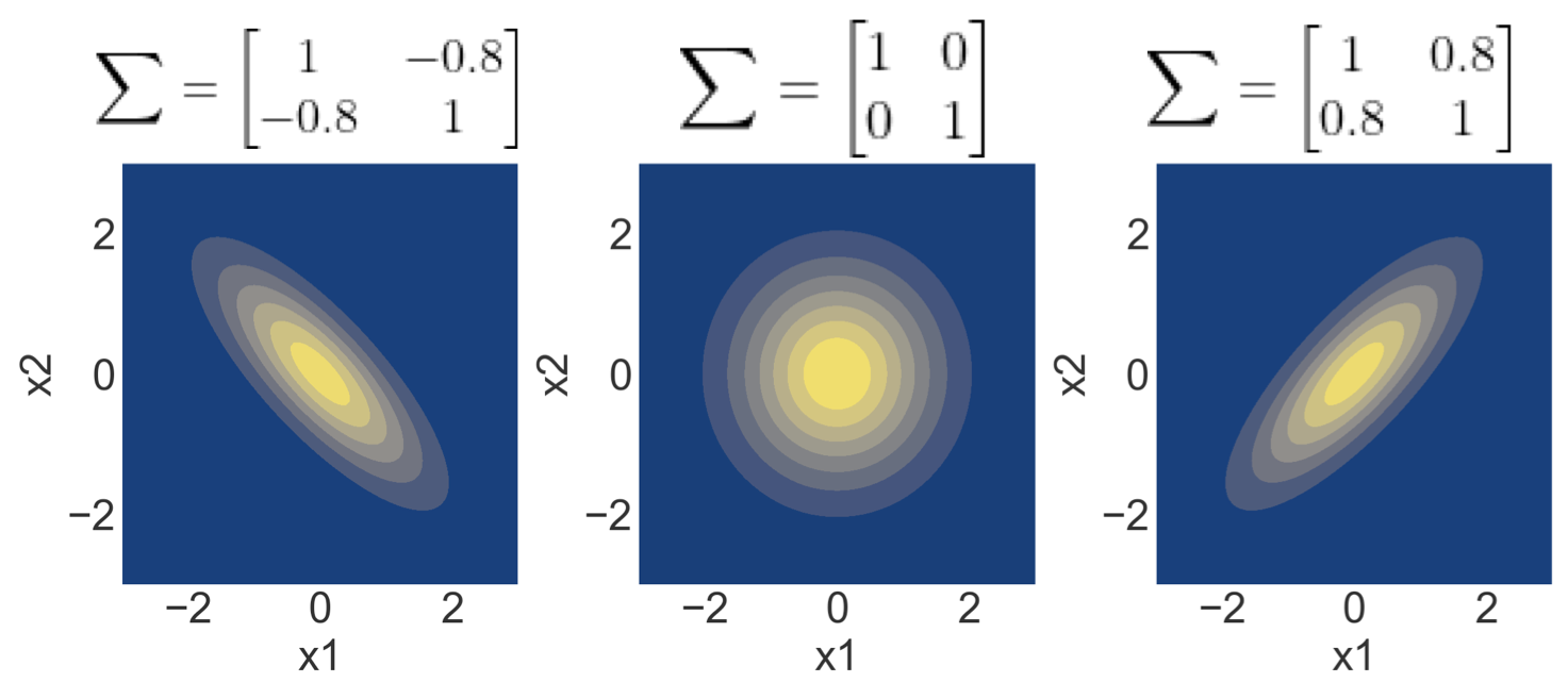
A 2D Gaussian example:
Here is an example of a 2D Gaussian distribution with mean 0, with the oval contours denoting points of constant probability.The covariance matrix, denoted as $\Sigma$, with the diagonal entries showing the variance of each individual random variable and the off-diagonal entries depicting the covariance between the random variables.
Partitioning
A Gaussian random vector $x\in\mathbb{R}^{n}$ with $x\sim\mathcal{N}(\mu,\Sigma)$ that can be partitioned into two subvectors $x_{A}\in\mathbb{R}^{p}$
and $x_{B}\in\mathbb{R}^{q}$ (where $p+q=n$) such that the joint distribution is:
We have the following properties:
- Normalization:
$$ \int _x p(x; \mu, \Sigma)dx=1 $$
-
Marginalization: The marginal distributions of $x_A$ and $x_B$ are Gaussian. Each partition $x_A$ and $x_B$ only depends on its corresponding entries in $\mu$ and $\Sigma$ $$ x_A \sim \mathcal{N}(\mu_A, \Sigma_{AA}) $$ $$ x_B \sim \mathcal{N}(\mu_B, \Sigma_{BB}) $$
-
Conditioning: The conditional distributions are also Gaussian with $$ x_A | x_B \sim \mathcal{N}(\mu_A + \Sigma_{AB}\Sigma_{BB}^{-1} (x_B-\mu_B), \Sigma_{AA}-\Sigma_{AB}\Sigma_{BB}^{-1}\Sigma_{BA} ) $$
$$ x_B | x_A \sim \mathcal{N}(\mu_B + \Sigma_{BA}\Sigma_{AA}^{-1} (x_A-\mu_A), \Sigma_{BB}-\Sigma_{BA}\Sigma_{AA}^{-1}\Sigma_{AB} ) $$
As can be seen that the new mean only depends on the conditioned variable, while the covariance matrix is independent from this variable.
From above its intutive to understand following: A GP is a (potentially infinte) collection of random variables (RV) such that the joint distribution of every finite subset of RVs is multivariate Gaussian: $$ f(x)\backsim GP(\mu(x),k(x,x^\prime)) $$ Like a Gaussian distribution is specified by its mean and variance, a Gaussian process is also completely defined by mean and covariance. Above, $\mu(x)$ is the mean and $k(x,x^\prime)$ is the covariance function. In a GP, we can derive the posterior from the prior and our observations. The predictive distribution $P(f_\ast|x_\ast,D) \sim \mathcal{N}(\mu_\ast,\Sigma_{\ast\ast})$ can be modeled using a prior $P(f|x,D) \sim \mathcal{N}(\mu,\Sigma)$ and condition it on the training data $D$ to model the joint distribution
 with $f=f(X)$ (vector of training observations) and $f_\ast=f(x_\ast)$ (prediction at test input). $\Sigma$ is denoted as $K$ for kernel because it’s computation will vary according to a kernel function.
Kernel Function
In GP, the covariance matrix is generated by evaluating the kernel k. The role of kernel is to describes the similarity between the observation, like the covariance matrix. Many of these kernels conceptually embed the input points into a higher dimensional space in which they then measure the similarity. Thus, we need to make sure that the resulting matrix adheres to the properties of a covariance matrix - should be positive definite. It controls the possible shape of the function.
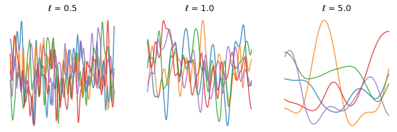
The most widely used kernel is probably the radial basis function kernel (also called the quadratic exponential kernel,
the squared exponential kernel or the Gaussian kernel):
$$
k(x,x^\prime)= \sigma^2exp\left(\frac{||x-x^\prime||^2}{2l^2} \right )
$$
Here, $l$ a length scale parameter that has significant effects. So with a Gaussian RBF kernel, any two points have positive correlation – but it goes to zero pretty quickly as one gets farther and farther away. For a smaller length scale, the function is allowed to change faster.
A few samples from the prior with SE kernel at different length-scales $l$.