Graph Based Classification on Protein Dataset
Posted on * • 5 minutes • 957 words
import torch
import torch.nn.functional as F
from torch.nn import Linear, Sequential, BatchNorm1d, ReLU, Dropout
!pip install -q git+https://github.com/pyg-team/pytorch_geometric.git
!pip install -q torch-scatter -f https://data.pyg.org/whl/torch-{torch.__version__}.html
!pip install -q torch-sparse -f https://data.pyg.org/whl/torch-{torch.__version__}.html
# Visualization
import networkx as nx
import matplotlib.pyplot as plt
plt.rcParams['figure.dpi'] = 50
plt.rcParams.update({'font.size': 24})
Data
from torch_geometric.datasets import TUDataset

dataset = TUDataset(root='.', name='PROTEINS').shuffle()

# Print information about the dataset
print(f'Dataset: {dataset}')
print('-------------------')
print(f'Number of graphs: {len(dataset)}')
print(f'Number of nodes: {dataset[0].x.shape[0]}')
print(f'Number of features: {dataset.num_features}')
print(f'Number of classes: {dataset.num_classes}')
Downloading https://www.chrsmrrs.com/graphkerneldatasets/PROTEINS.zip
Processing...


Dataset: PROTEINS(1113)
-------------------
Number of graphs: 1113
Number of nodes: 30
Number of features: 3
Number of classes: 2


Done!
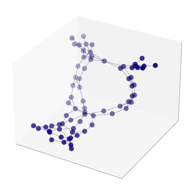
Visualise Data Example
from torch_geometric.utils import to_networkx
from mpl_toolkits.mplot3d import Axes3D
import numpy as np

G = to_networkx(dataset[2], to_undirected=True)

# 3D spring layout
pos = nx.spring_layout(G, dim=3, seed=0)

# Extract node and edge positions from the layout
node_xyz = np.array([pos[v] for v in sorted(G)])
edge_xyz = np.array([(pos[u], pos[v]) for u, v in G.edges()])

# Create the 3D figure
fig = plt.figure(figsize=(16,16))
ax = fig.add_subplot(111, projection="3d")

# Suppress tick labels
for dim in (ax.xaxis, ax.yaxis, ax.zaxis):
    dim.set_ticks([])

# Plot the nodes - alpha is scaled by "depth" automatically
ax.scatter(*node_xyz.T, s=500, c="#0A047A")

# Plot the edges
for vizedge in edge_xyz:
    ax.plot(*vizedge.T, color="tab:gray")

# fig.tight_layout()
plt.show()
from torch_geometric.loader import DataLoader

# Create training, validation, and test sets
train_dataset = dataset[:int(len(dataset)*0.8)]
val_dataset   = dataset[int(len(dataset)*0.8):int(len(dataset)*0.9)]
test_dataset  = dataset[int(len(dataset)*0.9):]

print(f'Training set   = {len(train_dataset)} graphs')
print(f'Validation set = {len(val_dataset)} graphs')
print(f'Test set       = {len(test_dataset)} graphs')

# Create mini-batches
train_loader = DataLoader(train_dataset, batch_size=64, shuffle=True)
val_loader = DataLoader(val_dataset, batch_size=64, shuffle=True)
test_loader = DataLoader(test_dataset, batch_size=64, shuffle=False)

print('\nTrain loader:')
for i, subgraph in enumerate(train_loader):
    print(f' - Subgraph {i}: {subgraph}')

print('\nValidation loader:')
for i, subgraph in enumerate(val_loader):
    print(f' - Subgraph {i}: {subgraph}')

print('\nTest loader:')
for i, subgraph in enumerate(test_loader):
    print(f' - Subgraph {i}: {subgraph}')
Training set   = 890 graphs
Validation set = 111 graphs
Test set       = 112 graphs

Train loader:
 - Subgraph 0: DataBatch(edge_index=[2, 9222], x=[2414, 3], y=[64], batch=[2414], ptr=[65])
 - Subgraph 1: DataBatch(edge_index=[2, 15440], x=[3923, 3], y=[64], batch=[3923], ptr=[65])
 - Subgraph 2: DataBatch(edge_index=[2, 9212], x=[2551, 3], y=[64], batch=[2551], ptr=[65])
 - Subgraph 3: DataBatch(edge_index=[2, 8962], x=[2379, 3], y=[64], batch=[2379], ptr=[65])
 - Subgraph 4: DataBatch(edge_index=[2, 10082], x=[2730, 3], y=[64], batch=[2730], ptr=[65])
 - Subgraph 5: DataBatch(edge_index=[2, 8712], x=[2324, 3], y=[64], batch=[2324], ptr=[65])
 - Subgraph 6: DataBatch(edge_index=[2, 9054], x=[2483, 3], y=[64], batch=[2483], ptr=[65])
 - Subgraph 7: DataBatch(edge_index=[2, 8142], x=[2207, 3], y=[64], batch=[2207], ptr=[65])
 - Subgraph 8: DataBatch(edge_index=[2, 9212], x=[2427, 3], y=[64], batch=[2427], ptr=[65])
 - Subgraph 9: DataBatch(edge_index=[2, 8920], x=[2426, 3], y=[64], batch=[2426], ptr=[65])
 - Subgraph 10: DataBatch(edge_index=[2, 7106], x=[1929, 3], y=[64], batch=[1929], ptr=[65])
 - Subgraph 11: DataBatch(edge_index=[2, 12000], x=[3318, 3], y=[64], batch=[3318], ptr=[65])
 - Subgraph 12: DataBatch(edge_index=[2, 9092], x=[2440, 3], y=[64], batch=[2440], ptr=[65])
 - Subgraph 13: DataBatch(edge_index=[2, 8696], x=[2353, 3], y=[58], batch=[2353], ptr=[59])

Validation loader:
 - Subgraph 0: DataBatch(edge_index=[2, 7838], x=[2042, 3], y=[64], batch=[2042], ptr=[65])
 - Subgraph 1: DataBatch(edge_index=[2, 5438], x=[1432, 3], y=[47], batch=[1432], ptr=[48])

Test loader:
 - Subgraph 0: DataBatch(edge_index=[2, 8724], x=[2368, 3], y=[64], batch=[2368], ptr=[65])
 - Subgraph 1: DataBatch(edge_index=[2, 6236], x=[1725, 3], y=[48], batch=[1725], ptr=[49])
from torch_geometric.nn import GCNConv, GINConv
from torch_geometric.nn import global_mean_pool, global_add_pool
GCN
class GCN(torch.nn.Module):
    """GCN"""
    def __init__(self, dim_h):
        super(GCN, self).__init__()
        self.conv1 = GCNConv(dataset.num_node_features, dim_h)
        self.conv2 = GCNConv(dim_h, dim_h)
        self.conv3 = GCNConv(dim_h, dim_h)
        self.lin = Linear(dim_h, dataset.num_classes)

    def forward(self, x, edge_index, batch):
        # Node embeddings
        h = self.conv1(x, edge_index)
        h = h.relu()
        h = self.conv2(h, edge_index)
        h = h.relu()
        h = self.conv3(h, edge_index)

        # Graph-level readout
        hG = global_mean_pool(h, batch)

        # Classifier
        h = F.dropout(hG, p=0.5, training=self.training)
        h = self.lin(h)

        return hG, F.log_softmax(h, dim=1)
gcn = GCN(dim_h=32)
GIN
class GIN(torch.nn.Module):
    """GIN"""
    def __init__(self, dim_h):
        super(GIN, self).__init__()
        self.conv1 = GINConv(
            Sequential(Linear(dataset.num_node_features, dim_h),
                       BatchNorm1d(dim_h), ReLU(),
                       Linear(dim_h, dim_h), ReLU()))
        self.conv2 = GINConv(
            Sequential(Linear(dim_h, dim_h), BatchNorm1d(dim_h), ReLU(),
                       Linear(dim_h, dim_h), ReLU()))
        self.conv3 = GINConv(
            Sequential(Linear(dim_h, dim_h), BatchNorm1d(dim_h), ReLU(),
                       Linear(dim_h, dim_h), ReLU()))
        self.lin1 = Linear(dim_h*3, dim_h*3)
        self.lin2 = Linear(dim_h*3, dataset.num_classes)

    def forward(self, x, edge_index, batch):
        # Node embeddings
        h1 = self.conv1(x, edge_index)
        h2 = self.conv2(h1, edge_index)
        h3 = self.conv3(h2, edge_index)

        # Graph-level readout
        h1 = global_add_pool(h1, batch)
        h2 = global_add_pool(h2, batch)
        h3 = global_add_pool(h3, batch)

        # Concatenate graph embeddings
        h = torch.cat((h1, h2, h3), dim=1)

        # Classifier
        h = self.lin1(h)
        h = h.relu()
        h = F.dropout(h, p=0.5, training=self.training)
        h = self.lin2(h)

        return h, F.log_softmax(h, dim=1)
gin = GIN(dim_h=32)
Train Models
def train(model, loader):
    criterion = torch.nn.CrossEntropyLoss()
    optimizer = torch.optim.Adam(model.parameters(),
                                      lr=0.01,
                                      weight_decay=0.01)
    epochs = 100

    model.train()
    for epoch in range(epochs+1):
        total_loss = 0
        acc = 0
        val_loss = 0
        val_acc = 0

        # Train on batches
        for data in loader:
          optimizer.zero_grad()
          _, out = model(data.x, data.edge_index, data.batch)
          loss = criterion(out, data.y)
          total_loss += loss / len(loader)
          acc += accuracy(out.argmax(dim=1), data.y) / len(loader)
          loss.backward()
          optimizer.step()

          # Validation
          val_loss, val_acc = test(model, val_loader)

    # Print metrics every 10 epochs
    if(epoch % 10 == 0):
        print(f'Epoch {epoch:>3} | Train Loss: {total_loss:.2f} '
              f'| Train Acc: {acc*100:>5.2f}% '
              f'| Val Loss: {val_loss:.2f} '
              f'| Val Acc: {val_acc*100:.2f}%')

    test_loss, test_acc = test(model, test_loader)
    print(f'Test Loss: {test_loss:.2f} | Test Acc: {test_acc*100:.2f}%')

    return model
def accuracy(pred_y, y):
    """Calculate accuracy."""
    return ((pred_y == y).sum() / len(y)).item()
@torch.no_grad()
def test(model, loader):
    criterion = torch.nn.CrossEntropyLoss()
    model.eval()
    loss = 0
    acc = 0

    for data in loader:
        _, out = model(data.x, data.edge_index, data.batch)
        loss += criterion(out, data.y) / len(loader)
        acc += accuracy(out.argmax(dim=1), data.y) / len(loader)

    return loss, acc
gcn = train(gcn, train_loader)
gin = train(gin, train_loader)
Epoch 100 | Train Loss: 0.51 | Train Acc: 76.43% | Val Loss: 0.59 | Val Acc: 71.33%
Test Loss: 0.58 | Test Acc: 73.44%
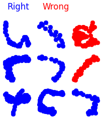
Visualize test results
fig, ax = plt.subplots(3, 3, figsize=(5,5))
fig.text(0.25,0.95,"Right", ha="center", va="bottom", size="medium",color="blue")
fig.text(0.55, 0.95, "Wrong", ha="center", va="bottom", size="medium",color="red")

for i, data in enumerate(dataset[1113-9:]):
    # Calculate color (green if correct, red otherwise)
    _, out = gin(data.x, data.edge_index, data.batch)
    color = "blue" if out.argmax(dim=1) == data.y else "red"

    # Plot graph
    ix = np.unravel_index(i, ax.shape)
    ax[ix].axis('off')
    G = to_networkx(dataset[i], to_undirected=True)
    nx.draw_networkx(G,
                    pos=nx.spring_layout(G, seed=0),
                    with_labels=False,
                    node_size=150,
                    node_color=color,
                    width=0.8,
                    ax=ax[ix]
                    )