NetworkX - Visualizing PytorchGeometric Datasets
Posted on * • 9 minutes • 1888 words
import networkx as nx
In NetworkX, nodes can be any hashable object (eg., text, image, an XML object, another graph, a customized node object)
NetworkX includes many graph generator functions and facilities to read and write graphs in many formats.
- add_node
- add_nodes_from
- add_edge
- add_edges_from
- remove_node etc..
Create a graph
G = nx.Graph()
# nx.draw(G) #=> will be empty canvas

# add one node at a time,
G.add_node(1)
# nx.draw(G)
# Add from a collection
G.add_nodes_from([2,3,4,5])
#nx.draw(G)
G.add_edge(5,1)
#nx.draw(G)
G.add_nodes_from([6,7,8])
G.add_edges_from([(6,7),(7,8), (1,4), (2,3), (3,6),(5,6)])
nx.draw(G)
print(f"Number of nodes = {G.number_of_nodes()}")
print(f"Number of edges = {G.number_of_edges()}")
print(G.edges)
print(G.nodes)
Number of nodes = 8
Number of edges = 7
[(1, 5), (1, 4), (2, 3), (3, 6), (5, 6), (6, 7), (7, 8)]
[1, 2, 3, 4, 5, 6, 7, 8]
Export graph as JSON
from networkx.readwrite import json_graph
json_data = json_graph.node_link_data(G)
json_data
{'directed': False,
 'multigraph': False,
 'graph': {},
 'nodes': [{'id': 1},
  {'id': 2},
  {'id': 3},
  {'id': 4},
  {'id': 5},
  {'id': 6},
  {'id': 7},
  {'id': 8}],
 'links': [{'source': 1, 'target': 5},
  {'source': 1, 'target': 4},
  {'source': 2, 'target': 3},
  {'source': 3, 'target': 6},
  {'source': 5, 'target': 6},
  {'source': 6, 'target': 7},
  {'source': 7, 'target': 8}]}
Read a json graph
json_data_to_graph = json_graph.node_link_graph(json_data)
json_data_to_graph
<networkx.classes.graph.Graph at 0x7e7f04523580>
Generate Graphml
for line in nx.generate_graphml(G):
  print(line)
<graphml xmlns="http://graphml.graphdrawing.org/xmlns" xmlns:xsi="http://www.w3.org/2001/XMLSchema-instance" xsi:schemaLocation="http://graphml.graphdrawing.org/xmlns http://graphml.graphdrawing.org/xmlns/1.0/graphml.xsd">
  <graph edgedefault="undirected">
    <node id="1" />
    <node id="2" />
    <node id="3" />
    <node id="4" />
    <node id="5" />
    <node id="6" />
    <node id="7" />
    <node id="8" />
    <edge source="1" target="5" />
    <edge source="1" target="4" />
    <edge source="2" target="3" />
    <edge source="3" target="6" />
    <edge source="5" target="6" />
    <edge source="6" target="7" />
    <edge source="7" target="8" />
  </graph>
</graphml>
Remove Nodes or Clear graph
G.remove_nodes_from([1,3])
G.clear()
More of it
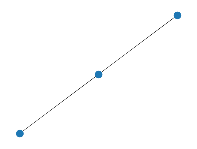
G.add_edges_from([(1,2),(1,3)])
print(G.edges())
print(G.nodes())
nx.draw(G)
[(1, 2), (1, 3)]
[1, 2, 3]
G.add_node("spam")       # adds node "spam"
G.add_nodes_from("spam") # adds 4 nodes: 's', 'p', 'a', 'm'
print(G.edges())
print(G.nodes())
#nx.draw(G)
[(1, 2), (1, 3)]
[1, 2, 3, 'spam', 's', 'p', 'a', 'm']
Order, Density and Degree of Graph
Order => number of nodes Density for undirected graph:
$$ d = \frac{2e}{n(n-1)} $$ where $n$ is the number of nodes and $e$ is the number of edges
Degree : Returns a degree view
# Number of Nodes
G.order()
8
from networkx.classes.function import density
density(G)
0.07142857142857142
from networkx.classes.function import degree
degree(G, nbunch=None, weight=None)
DegreeView({1: 2, 2: 1, 3: 1, 'spam': 0, 's': 0, 'p': 0, 'a': 0, 'm': 0})
# In above graph G, degreeview shows 5 0's; 2 1's and 1 2;s
from networkx.classes.function import degree_histogram
degree_histogram(G)
[5, 2, 1]
from networkx.classes.function import neighbors
neighbors(G, 'spam')
<dict_keyiterator at 0x7e7f0442e070>
for node in G.nodes():
  print(node, G.neighbors(node))
1 <dict_keyiterator object at 0x7e7f044dc400>
2 <dict_keyiterator object at 0x7e7f044dc400>
3 <dict_keyiterator object at 0x7e7f044dc400>
spam <dict_keyiterator object at 0x7e7f044dc400>
s <dict_keyiterator object at 0x7e7f044dc400>
p <dict_keyiterator object at 0x7e7f044dc400>
a <dict_keyiterator object at 0x7e7f044dc400>
m <dict_keyiterator object at 0x7e7f044dc400>
for node in G.nodes():
  print(node, list(G.neighbors(node)))
1 [2, 3]
2 [1]
3 [1]
spam []
s []
p []
a []
m []
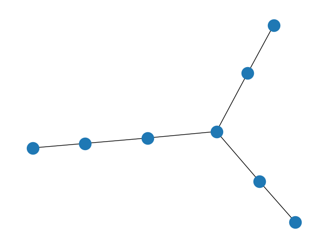
Graph Generators
https://networkx.org/documentation/stable/reference/generators.html
G.clear()
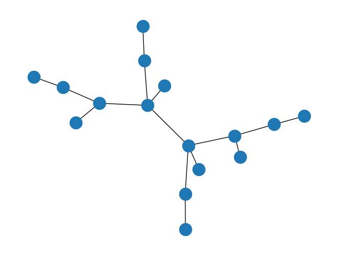
G = nx.binomial_tree(4)
nx.draw(G)
# default is 3x3 = 9 nodes
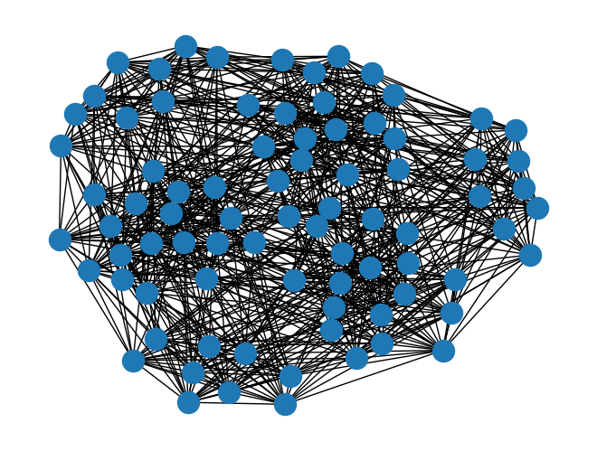
G = nx.sudoku_graph()
print(G.number_of_nodes())
print(G.number_of_edges())
print("--------------------")
A = nx.adjacency_matrix(G)
print(A.todense())
nx.draw(G)
81
810
--------------------
[[0 1 1 ... 0 0 0]
 [1 0 1 ... 0 0 0]
 [1 1 0 ... 0 0 0]
 ...
 [0 0 0 ... 0 1 1]
 [0 0 0 ... 1 0 1]
 [0 0 0 ... 1 1 0]]
Directed Graphs
Neighbor And Adjacency
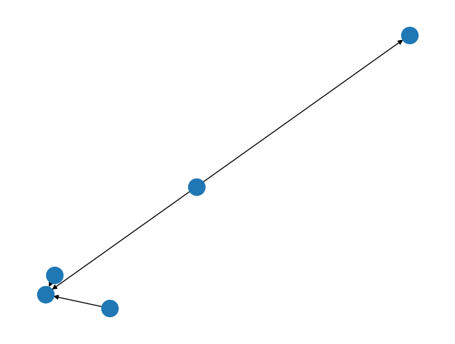
G = nx.DiGraph()
G.add_edge('a', 'b', weight=1)
G.add_edge('c', 'b', weight=5)
G.add_edge('m', 'n', weight=25)
G.add_edge('m', 'b', weight=50)
nx.draw(G)
print(nx.is_weighted(G))
print(nx.is_directed(G))
print(G.order())
print(G.number_of_edges())
print(G.number_of_nodes())
print(G.edges)
print(G.nodes)
True
True
5
4
5
[('a', 'b'), ('c', 'b'), ('m', 'n'), ('m', 'b')]
['a', 'b', 'c', 'm', 'n']
print([n for n in G.neighbors('a')])
print("===========")

for node in G.nodes():
  print(node, list(G.neighbors(node)))

print("===========")
print([n for n in G.neighbors('m')])
['b']
===========
a ['b']
b []
c ['b']
m ['n', 'b']
n []
===========
['n', 'b']
for x in G.nodes:
  print('Neighbors for ' + x + ':')
  print([n for n in G.neighbors(x)])
Neighbors for a:
['b']
Neighbors for b:
[]
Neighbors for c:
['b']
Neighbors for m:
['n', 'b']
Neighbors for n:
[]
A = nx.adjacency_matrix(G)
print(A)
print("====")
print(A.todense())
  (0, 1)	1
  (2, 1)	5
  (3, 1)	50
  (3, 4)	25
====
[[ 0  1  0  0  0]
 [ 0  0  0  0  0]
 [ 0  5  0  0  0]
 [ 0 50  0  0 25]
 [ 0  0  0  0  0]]
# Is it self-looped
A.diagonal()
array([0, 0, 0, 0, 0])
# From G to numpy array gives A
A = nx.to_numpy_array(G)
print(A)
[[ 0.  1.  0.  0.  0.]
 [ 0.  0.  0.  0.  0.]
 [ 0.  5.  0.  0.  0.]
 [ 0. 50.  0.  0. 25.]
 [ 0.  0.  0.  0.  0.]]
Multiple Edge Attributes
import numpy as np

G = nx.Graph()
G.add_edge(0, 1, weight=10)
G.add_edge(1, 2, cost=5)
G.add_edge(2, 3, weight=3, cost=-4.0)
dtype = np.dtype([("weight", int), ("cost", float)])
# To create adjacency matrices from structured dtypes, use `weight=None`
A = nx.to_numpy_array(G, dtype=dtype, weight=None)
print("weight --------")
print(A["weight"])
print("cost --------")
print(A["cost"])

print(G.edges)
print(G.nodes)
weight --------
[[ 0 10  0  0]
 [10  0  1  0]
 [ 0  1  0  3]
 [ 0  0  3  0]]
cost --------
[[ 0.  1.  0.  0.]
 [ 1.  0.  5.  0.]
 [ 0.  5.  0. -4.]
 [ 0.  0. -4.  0.]]
[(0, 1), (1, 2), (2, 3)]
[0, 1, 2, 3]
G = nx.Graph(
    [
        ("A", "B", {"cost": 1, "weight": 7}),
        ("C", "E", {"cost": 9, "weight": 10}),
    ]
)
print(G.edges)
print(G.nodes)
print("---------- #For entire graph ----------")
df = nx.to_pandas_edgelist(G)
print(df)

print("--------#for selected list BE------------")
df = nx.to_pandas_edgelist(G, nodelist=["B", "E"]) #for selected list
print(df)
print("--------------------")
df = nx.to_pandas_edgelist(G, nodelist=["A", "C"])
print(df)
print("--------------------")
df[["source", "target", "cost", "weight"]]
[('A', 'B'), ('C', 'E')]
['A', 'B', 'C', 'E']
---------- #For entire graph ----------
  source target  cost  weight
0      A      B     1       7
1      C      E     9      10
--------#for selected list BE------------
  source target  cost  weight
0      B      A     1       7
1      E      C     9      10
--------------------
  source target  cost  weight
0      A      B     1       7
1      C      E     9      10
--------------------
# Only weights
A = nx.adjacency_matrix(G)
print(A.todense())
[[ 0  7  0  0]
 [ 7  0  0  0]
 [ 0  0  0 10]
 [ 0  0 10  0]]
Viewing Datasets from Pytorch Geometry
1. Enzyme Dataset
!python -c "import torch; print(torch.__version__)"
2.1.0+cu121
!pip install torch-scatter -f https://data.pyg.org/whl/torch-2.1.0+cu121.html
!pip install torch-sparse -f https://data.pyg.org/whl/torch-2.1.0+cu121.html
!pip install torch-geometric
from torch_geometric.datasets import TUDataset
dataset = TUDataset(root='/tmp/ENZYMES', name='ENZYMES')
Downloading https://www.chrsmrrs.com/graphkerneldatasets/ENZYMES.zip
Processing...
Done!
print(f"{dataset} : {len(dataset)}")
print(f"Num classes : {dataset.num_classes}")
print(f"Num classes : {dataset.num_node_features}")
ENZYMES(600) : 600
Num classes : 6
Num classes : 3
data = dataset[0]
data
Data(edge_index=[2, 168], x=[37, 3], y=[1])
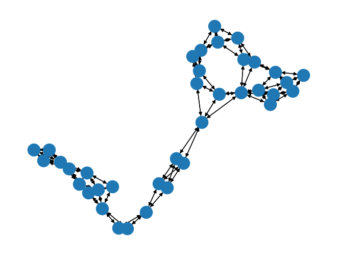
from torch_geometric.utils import to_networkx
print(type(data))

networkX_graph = to_networkx(data)
print(type(networkX_graph))
<class 'torch_geometric.data.data.Data'>
<class 'networkx.classes.digraph.DiGraph'>
import networkx as nx
nx.draw(networkX_graph)
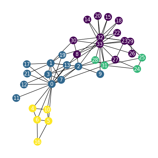
2. Karate Dataset
# Helper function for visualization.
%matplotlib inline
import matplotlib.pyplot as plt
from torch_geometric.datasets import KarateClub
dataset = KarateClub()
print(f'Dataset: {dataset}:')
print('======================')
print(f'Number of graphs: {len(dataset)}')
print(f'Number of features: {dataset.num_features}')
print(f'Number of classes: {dataset.num_classes}')
print(f'Number of Node Features: {dataset.num_node_features}')
print(f'Number of Edge Features: {dataset.num_edge_features}')
Dataset: KarateClub():
======================
Number of graphs: 1
Number of features: 34
Number of classes: 4
Number of Node Features: 34
Number of Edge Features: 0
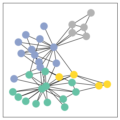
- This dataset holds exactly one graph,
- Each node in this dataset is assigned a 34-dimensional feature vector (which uniquely describes the members of the karate club).
- The graph holds exactly 4 classes, which represent the community each node belongs to.
data = dataset[0]  # Get the first graph object.
print(data)
# (1) The edge_index property holds the information about the graph connectivity, i.e., a tuple of source and destination node indices for each edge.
# (2) node features as x (each of the 34 nodes is assigned a 34-dim feature vector)
# (3) node labels as y (each node is assigned to exactly one class).
Data(x=[34, 34], edge_index=[2, 156], y=[34], train_mask=[34])
print('==============================================================')

# Gather some statistics about the graph.
print(f'Number of nodes: {data.num_nodes}')
print(f'Number of edges: {data.num_edges}')
print(f'Average node degree: {data.num_edges / data.num_nodes:.2f}')
print(f'Has isolated nodes: {data.has_isolated_nodes()}')
print(f'Has self-loops: {data.has_self_loops()}')
print(f'Is Directed: {data.is_directed()}')
print(f'Is undirected: {data.is_undirected()}')
print('==============================================================')

print(f'Edge weight: {data.edge_weight}')
print(f'Graph contains isolated nodes: {data.contains_isolated_nodes()}')

print('==============================================================')
print(f'Number of training nodes: {data.train_mask.sum()}')
print(f'Training node label rate: {int(data.train_mask.sum()) / data.num_nodes:.2f}')
==============================================================
Number of nodes: 34
Number of edges: 156
Average node degree: 4.59
Has isolated nodes: False
Has self-loops: False
Is Directed: False
Is undirected: True
==============================================================
Edge weight: None
Graph contains isolated nodes: False
==============================================================
Number of training nodes: 4
Training node label rate: 0.12


/usr/local/lib/python3.10/dist-packages/torch_geometric/deprecation.py:26: UserWarning: 'contains_isolated_nodes' is deprecated, use 'has_isolated_nodes' instead
  warnings.warn(out)
data.to_dict()
{'x': tensor([[1., 0., 0.,  ..., 0., 0., 0.],
         [0., 1., 0.,  ..., 0., 0., 0.],
         [0., 0., 1.,  ..., 0., 0., 0.],
         ...,
         [0., 0., 0.,  ..., 1., 0., 0.],
         [0., 0., 0.,  ..., 0., 1., 0.],
         [0., 0., 0.,  ..., 0., 0., 1.]]),
 'edge_index': tensor([[ 0,  0,  0,  0,  0,  0,  0,  0,  0,  0,  0,  0,  0,  0,  0,  0,  1,  1,
           1,  1,  1,  1,  1,  1,  1,  2,  2,  2,  2,  2,  2,  2,  2,  2,  2,  3,
           3,  3,  3,  3,  3,  4,  4,  4,  5,  5,  5,  5,  6,  6,  6,  6,  7,  7,
           7,  7,  8,  8,  8,  8,  8,  9,  9, 10, 10, 10, 11, 12, 12, 13, 13, 13,
          13, 13, 14, 14, 15, 15, 16, 16, 17, 17, 18, 18, 19, 19, 19, 20, 20, 21,
          21, 22, 22, 23, 23, 23, 23, 23, 24, 24, 24, 25, 25, 25, 26, 26, 27, 27,
          27, 27, 28, 28, 28, 29, 29, 29, 29, 30, 30, 30, 30, 31, 31, 31, 31, 31,
          31, 32, 32, 32, 32, 32, 32, 32, 32, 32, 32, 32, 32, 33, 33, 33, 33, 33,
          33, 33, 33, 33, 33, 33, 33, 33, 33, 33, 33, 33],
         [ 1,  2,  3,  4,  5,  6,  7,  8, 10, 11, 12, 13, 17, 19, 21, 31,  0,  2,
           3,  7, 13, 17, 19, 21, 30,  0,  1,  3,  7,  8,  9, 13, 27, 28, 32,  0,
           1,  2,  7, 12, 13,  0,  6, 10,  0,  6, 10, 16,  0,  4,  5, 16,  0,  1,
           2,  3,  0,  2, 30, 32, 33,  2, 33,  0,  4,  5,  0,  0,  3,  0,  1,  2,
           3, 33, 32, 33, 32, 33,  5,  6,  0,  1, 32, 33,  0,  1, 33, 32, 33,  0,
           1, 32, 33, 25, 27, 29, 32, 33, 25, 27, 31, 23, 24, 31, 29, 33,  2, 23,
          24, 33,  2, 31, 33, 23, 26, 32, 33,  1,  8, 32, 33,  0, 24, 25, 28, 32,
          33,  2,  8, 14, 15, 18, 20, 22, 23, 29, 30, 31, 33,  8,  9, 13, 14, 15,
          18, 19, 20, 22, 23, 26, 27, 28, 29, 30, 31, 32]]),
 'y': tensor([1, 1, 1, 1, 3, 3, 3, 1, 0, 1, 3, 1, 1, 1, 0, 0, 3, 1, 0, 1, 0, 1, 0, 0,
         2, 2, 0, 0, 2, 0, 0, 2, 0, 0]),
 'train_mask': tensor([ True, False, False, False,  True, False, False, False,  True, False,
         False, False, False, False, False, False, False, False, False, False,
         False, False, False, False,  True, False, False, False, False, False,
         False, False, False, False])}
from IPython.display import Javascript  # Restrict height of output cell.
display(Javascript('''google.colab.output.setIframeHeight(0, true, {maxHeight: 300})'''))
<IPython.core.display.Javascript object>
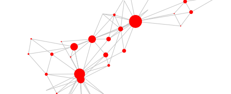
def visualize_graph(G, color):
    plt.figure(figsize=(5,5))
    plt.xticks([])
    plt.yticks([])
    nx.draw_networkx(G, pos=nx.spring_layout(G, seed=42), with_labels=False,
                     node_color=color, cmap="Set2")
    plt.show()

karate_undirected_graph = to_networkx(data, to_undirected=True)
visualize_graph(karate_undirected_graph, color=data.y)
plt.figure(figsize=(5,5))
nx.draw(karate_undirected_graph, cmap=plt.get_cmap('viridis'), with_labels=True, node_color=data.y, font_color='white')
# 4 Classes are visible