
PINNS - Physics in Neural Networks
Posted on * • 3 minutes • 490 words
Neural Networks are Function Approximators
According to the Universal Approximation Theorem, the Neural Networks (NN) with non-linear activations can approximate any function when given appropriate weights. It is important to note that the theorem is based on approximation error only. It does not say anyhting about its trainability. The network may need large number of neurons and millions of parameters and a lot of comutational resources. Anothe aspect is the generalizability, which require lots of data.
A Neural Network learns the function by minimising a loss function - the mean squared error (MSE) between its predictions $(\hat{u}_i)$ and the $(u_i)$
$$ \min_{\theta} \mathcal{L}_u = \sum||\hat{u}_i - u_i||_2 $$
The PINN approach is slightly different from the standard NN approach. Instead of relying purely on data, which could be limited, it uses the known partial differential equations (PDE) of the system to further guide the learning through the physics-based loss function i.e., just add the PDE residual as a soft constraint to the loss function when training the neural network. This way PINNs provide an alternative solution to the standard Finite elements modeling (FEM) methods.
Hypothetical Example
Lets assume a process where underlying physics can be described by the following differential equation: $$ a \frac{d^2y}{dx^2} + b \frac{dy}{dx} + cy = 0 $$ with boundary conditions $y(0) = y0$ and $y(1) = y1$.
The componenets of the loss function that has to minimized would be:
$$ \min(\mathcal{L}_u + \mathcal{L}_r + \mathcal{L}_b) $$
where,
- Data Loss Function: $$ \mathcal{L}_u = \sum||\hat{u}_i - u_i||_2 $$
- Physics based Loss Function:
Residual of the Differential Equation:
$$ \mathcal{L}_r = \left[ a \frac{d^2y}{dx^2} + b \frac{dy}{dx} + cy - 0\right]^{2} $$
and Boundary Condiitons
$$ \mathcal{L}_{b} = \left[ (\hat{y}(0) - y0)^2 + (\hat{y}(1) - y1)^2 \right] $$
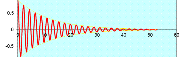
Damped Harmonic Oscillator
 Image from https://benmoseley.blog/
The dynmaics of a Damped Oscillator can be described by the following differential equation: $$ m \frac{d^2u}{dx^2} + \mu \frac{du}{dx} + ku = 0 $$ Where $m$ is the mass of the oscillator, $\mu$ is the coefficient of friction and $k$ is the spring constant. The physics loss in this case can be given by:
$$ \frac{1}{M}\sum_{j}^{M} \left(\left[m \frac{d^2}{dx^2} + \mu \frac{d}{dx} + k \right]\hat{y}_j\right) $$
Can be easily implemented in Pytorch, where x_data are the limited data points and x_physics represents the data points over the problem domain,
and model is a two-layered netowrk with hyperbolic tangent activation followed by a dense layer.
#=== compute the "data loss" ===
yh = model(x_data)
loss1 = torch.mean((yh-y_data)**2)# use mean squared error

#=== compute the "physics loss" ===
yhp = model(x_physics)
# computes dy/dx
dx  = torch.autograd.grad(yhp, x_physics, torch.ones_like(yhp), create_graph=True)[0]
# computes d^2y/dx^2
dx2 = torch.autograd.grad(dx,  x_physics, torch.ones_like(dx),  create_graph=True)[0]
# computes the residual of the DHO differential equation
physics = dx2 + mu*dx + k*yhp
loss2 = (1e-4)*torch.mean(physics**2)

# backpropagate joint loss
loss = loss1 + loss2
loss.backward()
Reference / Further Reading
Karniadakis et.al. 2021 Nat. Rev. Phys.