Solubility Prediction using GNN
Posted on * • 7 minutes • 1399 words
We will use ESOL dataset and train GNN model to predict solubility directly from chemical structures
! pip install rdkit-pypi
!python -c "import torch; print(torch.__version__)"
2.1.0+cu121
!pip install torch-scatter -f https://data.pyg.org/whl/torch-2.1.0+cu121.html
!pip install torch-sparse -f https://data.pyg.org/whl/torch-2.1.0+cu121.html
!pip install torch-geometric
Dataset
import rdkit
from torch_geometric.datasets import MoleculeNet

# Load the ESOL dataset
data = MoleculeNet(root=".", name="ESOL")
data
Downloading https://deepchemdata.s3-us-west-1.amazonaws.com/datasets/delaney-processed.csv
Processing...
Done!

ESOL(1128)
# Investigating the dataset
print("Dataset type: ", type(data))
print("Dataset features: ", data.num_features)
print("Dataset target: ", data.num_classes)
print("Dataset length: ", data.len())
print("Sample  nodes: ", data[0].num_nodes)
print("Sample  edges: ", data[0].num_edges)
Dataset type:  <class 'torch_geometric.datasets.molecule_net.MoleculeNet'>
Dataset features:  9
Dataset target:  734
Dataset length:  1128
Sample  nodes:  32
Sample  edges:  68
print("Dataset sample: ", data[0])
Dataset sample: Data(x=[32, 9], edge_index=[2, 68], edge_attr=[68, 3], smiles='OCC3OC(OCC2OC(OC(C#N)c1ccccc1)C(O)C(O)C2O)C(O)C(O)C3O ', y=[1, 1])
# Look at features
data[0].x
tensor([[8, 0, 2, 5, 1, 0, 4, 0, 0],
        [6, 0, 4, 5, 2, 0, 4, 0, 0],
        [6, 0, 4, 5, 1, 0, 4, 0, 1],
        [8, 0, 2, 5, 0, 0, 4, 0, 1],
        [6, 0, 4, 5, 1, 0, 4, 0, 1],
        [8, 0, 2, 5, 0, 0, 4, 0, 0],
        [6, 0, 4, 5, 2, 0, 4, 0, 0],
        [6, 0, 4, 5, 1, 0, 4, 0, 1],
        [8, 0, 2, 5, 0, 0, 4, 0, 1],
        [6, 0, 4, 5, 1, 0, 4, 0, 1],
        [8, 0, 2, 5, 0, 0, 4, 0, 0],
        [6, 0, 4, 5, 1, 0, 4, 0, 0],
        [6, 0, 2, 5, 0, 0, 2, 0, 0],
        [7, 0, 1, 5, 0, 0, 2, 0, 0],
        [6, 0, 3, 5, 0, 0, 3, 1, 1],
        [6, 0, 3, 5, 1, 0, 3, 1, 1],
        [6, 0, 3, 5, 1, 0, 3, 1, 1],
        [6, 0, 3, 5, 1, 0, 3, 1, 1],
        [6, 0, 3, 5, 1, 0, 3, 1, 1],
        [6, 0, 3, 5, 1, 0, 3, 1, 1],
        [6, 0, 4, 5, 1, 0, 4, 0, 1],
        [8, 0, 2, 5, 1, 0, 4, 0, 0],
        [6, 0, 4, 5, 1, 0, 4, 0, 1],
        [8, 0, 2, 5, 1, 0, 4, 0, 0],
        [6, 0, 4, 5, 1, 0, 4, 0, 1],
        [8, 0, 2, 5, 1, 0, 4, 0, 0],
        [6, 0, 4, 5, 1, 0, 4, 0, 1],
        [8, 0, 2, 5, 1, 0, 4, 0, 0],
        [6, 0, 4, 5, 1, 0, 4, 0, 1],
        [8, 0, 2, 5, 1, 0, 4, 0, 0],
        [6, 0, 4, 5, 1, 0, 4, 0, 1],
        [8, 0, 2, 5, 1, 0, 4, 0, 0]])
# Investigating the edges in sparse COO format
data[0].edge_index.t()
tensor([[ 0,  1],
        [ 1,  0],
        [ 1,  2],
        [ 2,  1],
        [ 2,  3],
        [ 2, 30],
        [ 3,  2],
        [ 3,  4],
        [ 4,  3],
        [ 4,  5],
        [ 4, 26],
        [ 5,  4],
        [ 5,  6],
        [ 6,  5],
        [ 6,  7],
        [ 7,  6],
        [ 7,  8],
        [ 7, 24],
        [ 8,  7],
        [ 8,  9],
        [ 9,  8],
        [ 9, 10],
        [ 9, 20],
        [10,  9],
        [10, 11],
        [11, 10],
        [11, 12],
        [11, 14],
        [12, 11],
        [12, 13],
        [13, 12],
        [14, 11],
        [14, 15],
        [14, 19],
        [15, 14],
        [15, 16],
        [16, 15],
        [16, 17],
        [17, 16],
        [17, 18],
        [18, 17],
        [18, 19],
        [19, 14],
        [19, 18],
        [20,  9],
        [20, 21],
        [20, 22],
        [21, 20],
        [22, 20],
        [22, 23],
        [22, 24],
        [23, 22],
        [24,  7],
        [24, 22],
        [24, 25],
        [25, 24],
        [26,  4],
        [26, 27],
        [26, 28],
        [27, 26],
        [28, 26],
        [28, 29],
        [28, 30],
        [29, 28],
        [30,  2],
        [30, 28],
        [30, 31],
        [31, 30]])
from rdkit import Chem
from rdkit.Chem.Draw import IPythonConsole
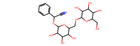
molecule = Chem.MolFromSmiles(data[0]["smiles"])
molecule
Graph Neural Network
import torch
from torch.nn import Linear
import torch.nn.functional as F
from torch_geometric.nn import GCNConv, TopKPooling, global_mean_pool
from torch_geometric.nn import global_mean_pool as gap, global_max_pool as gmp
embedding_size = 64

class GCN(torch.nn.Module):
    def __init__(self):
        # Init parent
        super(GCN, self).__init__()
        torch.manual_seed(42)

        # GCN layers
        self.initial_conv = GCNConv(data.num_features, embedding_size)
        self.conv1 = GCNConv(embedding_size, embedding_size)
        self.conv2 = GCNConv(embedding_size, embedding_size)
        self.conv3 = GCNConv(embedding_size, embedding_size)

        # Output layer
        self.out = Linear(embedding_size*2, 1)

    def forward(self, x, edge_index, batch_index):
        # First Conv layer
        hidden = self.initial_conv(x, edge_index)
        hidden = F.tanh(hidden)

        # Other Conv layers
        hidden = self.conv1(hidden, edge_index)
        hidden = F.tanh(hidden)
        hidden = self.conv2(hidden, edge_index)
        hidden = F.tanh(hidden)
        hidden = self.conv3(hidden, edge_index)
        hidden = F.tanh(hidden)

        # Global Pooling (stack different aggregations)
        hidden = torch.cat([gmp(hidden, batch_index),
                            gap(hidden, batch_index)], dim=1)

        # Apply a final (linear) classifier.
        out = self.out(hidden)

        return out, hidden
model = GCN()
print(model)
GCN(
  (initial_conv): GCNConv(9, 64)
  (conv1): GCNConv(64, 64)
  (conv2): GCNConv(64, 64)
  (conv3): GCNConv(64, 64)
  (out): Linear(in_features=128, out_features=1, bias=True)
)
Train
from torch_geometric.data import DataLoader
import warnings
warnings.filterwarnings("ignore")

# Root mean squared error
loss_fn = torch.nn.MSELoss()
optimizer = torch.optim.Adam(model.parameters(), lr=0.0007)

# Use GPU for training
device = torch.device("cuda:0" if torch.cuda.is_available() else "cpu")
model = model.to(device)

# Wrap data in a data loader
data_size = len(data)
NUM_GRAPHS_PER_BATCH = 64
loader = DataLoader(data[:int(data_size * 0.8)],
                    batch_size=NUM_GRAPHS_PER_BATCH, shuffle=True)
test_loader = DataLoader(data[int(data_size * 0.8):],
                         batch_size=NUM_GRAPHS_PER_BATCH, shuffle=True)

def train(data):
    # Enumerate over the data
    for batch in loader:
      # Use GPU
      batch.to(device)
      # Reset gradients
      optimizer.zero_grad()
      # Passing the node features and the connection info
      pred, embedding = model(batch.x.float(), batch.edge_index, batch.batch)
      # Calculating the loss and gradients
      loss = loss_fn(pred, batch.y)
      loss.backward()
      # Update using the gradients
      optimizer.step()
    return loss, embedding

print("Starting training...")
losses = []
for epoch in range(1000):
    loss, h = train(data)
    losses.append(loss)
    if epoch % 100 == 0:
      print(f"Epoch {epoch} | Train Loss {loss}")
Starting training...
Epoch 0 | Train Loss 0.7323977947235107
Epoch 100 | Train Loss 0.5643615126609802
Epoch 200 | Train Loss 0.8129488825798035
Epoch 300 | Train Loss 0.5515668988227844
Epoch 400 | Train Loss 0.26473188400268555
Epoch 500 | Train Loss 0.3548230826854706
Epoch 600 | Train Loss 0.10742906481027603
Epoch 700 | Train Loss 0.29880979657173157
Epoch 800 | Train Loss 0.08752292394638062
Epoch 900 | Train Loss 0.0839475765824318
Predictions
import pandas as pd
# Analyze the results for one batch
test_batch = next(iter(test_loader))
with torch.no_grad():
    test_batch.to(device)
    pred, embed = model(test_batch.x.float(), test_batch.edge_index, test_batch.batch)
    df = pd.DataFrame()
    df["y_real"] = test_batch.y.tolist()
    df["y_pred"] = pred.tolist()
df["y_real"] = df["y_real"].apply(lambda row: row[0])
df["y_pred"] = df["y_pred"].apply(lambda row: row[0])
df
| y_real | y_pred | |
|---|---|---|
| 0 | -1.300 | -1.867198 |
| 1 | -3.953 | -4.592132 |
| 2 | -3.091 | -3.610150 |
| 3 | -2.210 | -2.107021 |
| 4 | -5.850 | -4.743058 |
| ... | ... | ... |
| 59 | -4.522 | -4.377628 |
| 60 | -4.286 | -1.482177 |
| 61 | -3.900 | -3.672484 |
| 62 | -5.060 | -4.966655 |
| 63 | -7.200 | -7.057222 |
64 rows × 2 columns
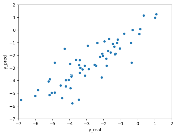
plt = sns.scatterplot(data=df, x="y_real", y="y_pred")
plt.set(xlim=(-7, 2))
plt.set(ylim=(-7, 2))
plt