Expectation Maximization and Gaussian Mixture Models
Posted on * • 5 minutes • 983 words
Expectation Maximization (EM)
Maximum Likelihood Estimation involves treating the problem as an optimization or search problem where one sets partial derivatives with respect to the parameters of the likelihood is zero and solves them. When these set of equations cannot be solved analytically - EM algorithm defines an iterative process that allows to maximize the likelihood function of a parametric model in the case in which some variables of the model are (or are treated as) “latent” or unknown.
Expectation-Maximization algorithm aims to use the observed data to estimate the latent variables and then using that to update the values of the parameters in the maximization step. The iterative approach cycles mainly between two steps:
- Expectation (E) Step. Estimate the missing/latent variables in the dataset.
- Maximization (M) Step. Maximize the parameters of the model in the presence of entire data (observed and latent).
A very common application of the EM method is fitting a mixture model.
Gaussian Mixtures
- Linear superposition of Gaussians
$$ P(x) = \sum_{k=1}^{K}\pi_k \mathcal{N}\left(x | \mu_k, \Sigma_k \right) $$
-
Normalization and positiovity rule $$ \sum_{k=1}^{K} \pi_k = 1 ;: 0 \leq pi_k \leq 1$$
-
Can interpret mixing co-efficients as prior probabilities
$$ P(x) = \sum_{k=1}^{K}P(k)P(x|k) $$
Fitting Gaussian Mixture
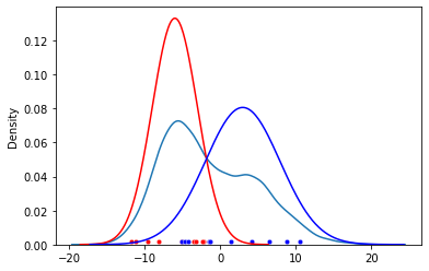
Mixture models in 1-d
We have observations $x_1, x_2, …, x_n$. Assume these come from two Gaussians ($K=2$, which is the latent variable/ latent component) with unknown parameters ($\mu$, $\sigma^{2}$). Figure below shows these observations as dots.
Case 1 - known source, unknown paramters
We know which observation is from which Gaussian (or which latent component), then estimating the parameter is trivial. With b for blue:
$$\mu_b = \frac{x_1 + x_2 + … + {x_{n}}_{b}}{n_b}$$ $$ \sigma^{2}_b = \frac{(x_1 - \mu_b)^2 + … + ({x_{n}}_{b} - \mu_b)^2}{n_b} $$
Case 2 - unknown source, known parameters
If we know the parameters of Gaussians, we can guess whether the point is more likely to be red ($r$) or blue ($b$).
$$ P(b|x_i) = \frac{P(x_i|b)P(b} {P(x_i|b)P(b) + P(x_i|r)P(r)} $$ $$ P(x_i|b) = \frac{1}{\sqrt{2\pi\sigma^2_2}} exp\left( -\frac{(x_i - \mu_b)^2}{2\sigma^2_b} \right) $$
Case 3 - unknown source, unknown parameters
Implement the expectation-maximization (EM) algorithm for fitting mixture-of-Gaussian models by an iterative process - a numerical technique for maximum likelihood estimation. It can be shown that the maximum likelihood of the data strictly increases with each subsequent iteration and thus is gauranteed to approach local maximum or saddle point.
Posterior Probabilties
- think of the mixing coefficients ($\pi_k$) as prior probabilities for the components
- For a given value of we can evaluate the corresponding posterior probabilities, called responsibilities. It is ratio of the Probability that $x_i$ dbelongs to class $k$ w.r.t its probability over all the classes. It can be given from Bayes theorem by
$$ \gamma_{ik} \equiv P(k|x) = \frac {P(k)P(x|k)} {P(x)} = \frac {\pi_k \mathcal{N}(x_i|\mu_k, \Sigma_{k})} {\sum_{j=1}^{K} \pi_j \mathcal{N}(x_i|\mu_j, \Sigma_{j})} $$
which is genralized form of Case 2 above. And, the multivariate gaussian is given by, $$ \mathcal{N}(x_i|\mu_k, \Sigma_{k}) = \frac{1}{\sqrt{(2\pi)^n|\Sigma_k|}} exp\left(-\frac{1}{2}(x_i - \mu_k)^T \Sigma_k^{-1}(x_i - \mu_k)\right) $$
Maximum Likelihood
The log likelihood will be: $$ ln P(X|\pi,\mu,\Sigma) = \sum_{i=1}^{N} ln \left( \sum_{k=1}^{K} \pi_k \mathcal{N}(x_i|\mu_k, \Sigma_k)\right) $$
Here sum over components appears inside the log. There is no closed form solution for the given maximum likelihood. The maximization of the log likelihood is solved by expectation-maximization (EM) algorithm.
GMM with Expectation-Maximization
Step one:
- Decide the number of clusters $(k)$.
- Initialize the means $\mu_k$, covariances $\Sigma_k$ , and mixing co-efficients $\pi_k$.
Step two: the E Step:
Calculate responsibilities $\gamma_{ik}$ using the current paramter values
Step three: the M - Step:
Once we computed $\gamma_{ik}$ we can comute the expexcted likelihood.
Re-estimate the parameters using the current responsibilities. Solving for $\mu_k$ and $\Sigma_k$ is like fitting $k$ separate Gaussians but with weighted by responsibilities $\gamma_{ik}$
$$ \pi_k = \frac{N_k}{N}$$ with $$ N_k = \sum_{n=1}^{N}\gamma_{ik}$$
$$ \mu_k = \frac{1}{N_k} \sum_{n=1}^{N} \gamma_{ik}x_i$$
$$ \Sigma_k = \frac{1}{N_k} \sum_{n=1}^{N} \gamma_{ik}(x_i - \mu_k)(x_i - \mu_k)^T $$
Step four:
If there is no convergence, return to Step 2. The entire iterative process repeats until the algorithm converges,
Nuts and Bolts in Python
Assume we have a dataset and we would like to know the parameters that generated the data (the source).
import numpy as np
from sklearn.datasets import make_blobs
from scipy.stats import multivariate_normal
We will generate a small toy data with 10 data points in 3 clusters. At this point we know 3 clusters, but it will be a latent variable.
n_samples = 10
centers = [[5, 5], [10, 15], [10,10]]
X, y = make_blobs(n_samples=n_samples, centers=centers, random_state=40)
-
Step 1 - Initialization
Assume number of sources equals 3. Radnomly initialize the mean taking random points from data, the covariance and pi.
number_of_sources = len(centers)
mu = (X[1,:]), (X[5,:]), (X[7,:])
mu = np.vstack(mu)

cov =[ np.cov(X.T) for _ in range(number_of_sources) ]

pi = np.ones(number_of_sources)/number_of_sources
-
Step 2 - The E-step
r_ik = np.zeros((n_samples, number_of_sources))

numerator = np.zeros( (n_samples, number_of_sources) )

for i in range(number_of_sources):
    r_ik[:,i] = multivariate_normal(mean=mu[i], cov=cov[i]).pdf(X)

denominator = r_ik.sum(axis=1)[:, np.newaxis]
r_ik = r_ik/denominator
At start r_ik was initialized with zeros. It indicates the probaility of each point being in the $k$th cluster and now is updated to :
r_ik -> array([[0.06244909, 0.1723533 , 0.76519761],
           [0.29184368, 0.47038617, 0.23777014],
           [0.47965241, 0.37006151, 0.15028608],
           [0.21491568, 0.43439897, 0.35068535],
           [0.48169748, 0.36806621, 0.15023631],
           [0.06380228, 0.20367482, 0.73252291],
           [0.16457573, 0.30695706, 0.52846721],
           [0.15749558, 0.29092674, 0.55157767],
           [0.29121053, 0.49204326, 0.21674621],
           [0.47990079, 0.3772105 , 0.14288871]])
-
Step 3 - The M-step
for i in range(number_of_sources):
    n_k = np.sum(r_ik[:,i],axis=0)
    mu[i] = (X * r_ik[:,[i]]).sum(axis=0) / n_k
    cov[i] = np.cov(X.T, aweights=(r_ik[:,[i]]/n_k).flatten(), bias=True)
Lets check cov before Step 3.
cov ->  [[ 8.37125986, 11.51406819],
            [11.51406819, 21.45486335]],
        [[ 8.37125986, 11.51406819],
            [11.51406819, 21.45486335]],
        [[ 8.37125986, 11.51406819],
            [11.51406819, 21.45486335]])]
The cov upon updation in Step 3.
cov ->  [[ 8.27448744, 12.41384471],
            [12.41384471, 19.94215921]],
        [[3.75845268, 4.72081764],
            [4.72081764, 9.81335957]]),
        [[ 2.63642289,  5.09967171],
            [ 5.09967171, 14.96354268]]
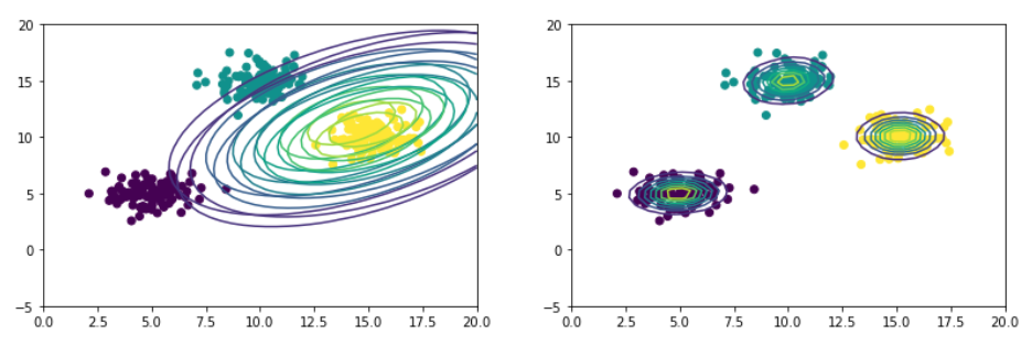
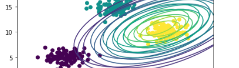
Large number of data points
The above set of steps were run on data with 300 points. Figure on left shows gaussians at the start and on right after 50 iterations.