Gibbs Sampling
Posted on * • 2 minutes • 412 words
Gibbs Sampling
Gibbs sampling is a Markov Chain Monte Carlo algorithm and a special case of the Metropolis-Hastings algorithm.
Gibbs Sampler can draw samples from any distribution, The Gibbs sampler draws iteratively from posterior conditional distributions rather than drawing directly from the joint posterior distribution. So it is useful in cases where joint distributions may be complex but one may be able to sample directly from less complicated conditional distributions.
Starting values are needed to initiate the Gibbs sampling process.The sampling depends on the values in the previous iteration; however, the sampling procedure is known to converge on to the final distribution, desired posterior, and that the process does on depend on the initial starting values.
Example: Bivariate Normal Distribution
With $\textbf{x} = (x_1, x_2)$, $\mu = (\mu_1, \mu_2)$ and $\Sigma$ being a $2 × 2$ covariance matrix with diagonal entries $\sigma_{1}^2$, $\sigma_{2}^2$ and off-diagonals $\sigma_{1,2}$.
- The pdf is
$$f(\textbf{x} | \mu,\Sigma) \propto \left| \Sigma \right|^{-1/2}exp\left( -\frac{1}{2}(\textbf{x} - \mu)^{t} \Sigma^{-1}(\textbf{x}-\mu) \right)$$
-
The Marginal distributions are given by $x_1 \sim N(\mu_1, \sigma_{1}^2)$ and $x_2 \sim N(\mu_2, \sigma_{2}^2)$
-
The conditionals, for Gibbs sampling, are given by:
$$f(x_1 | x_2) = N(\mu_1 + (\sigma_{1,2}/\sigma_{2}^2)(x_2 - \mu_2), \sigma_{1}^2 -(\sigma_{1,2}/ \sigma_{2})^{2} )$$ and, $$f(x_2 | x_1) = N(\mu_2 + (\sigma_{1,2}/\sigma_{1}^2)(x_1 - \mu_1), \sigma_{2}^2 -(\sigma_{1,2} / \sigma_{1})^{2} )$$
Python Implementation
Following is python implementation of Gibbs Sampling in case of 2D Gaussian distribution
def gibbs_sampling(joint_mu, joint_cov):
    def conditional_sampler(point, var_index):
        A = joint_cov[var_index, var_index]
        B = joint_cov[var_index, ~var_index]  #
        C = joint_cov[~var_index, ~var_index]
        mu = joint_mu[var_index] + B / C * (point[~var_index] - joint_mu[~var_index])
        sigma = A - B / C * B
        return np.random.normal(mu, sigma)
    return conditional_sampler

joint_mu = np.array([0, 1])
joint_cov = np.array([[1, -0.8], [-0.8, 1.5]])
sampler = gibbs_sampling(joint_mu, joint_cov)
define function that takes an inital point and number of smaples.
def generate_samples(initial_point, num_samples):
    point = np.array(initial_point)
    samples = np.zeros((num_samples, 2))
    samples[0] = point

    for i in range(1, num_samples):
        samples[i, :] = samples[i - 1, :]
        d = i % 2  #alternate between x2 and x1
        x = sampler(samples[i], d)
        samples[i,d] = x
    return samples
The main call - choose an initial point and call generate_samples
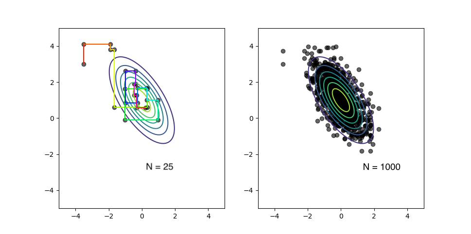
initial_point = [-3.5, 3.0]
num_samples = 25
samples = generate_samples(initial_point, num_samples)
Plottting generated samples
The figure on left shows the path taken by the generated samples, the next point depending on pevious one. As can be seen from the right panel, after a lot of iteration ($N = 1000$), it then converges to approximately the exact distribution being sampled.